Part Of: [Advanced Inference In Graphical Models] sequence

Table Of Contents

• Definitions Make The World Go ‘Round
• Searching The Universe
• The Topography Of Truth
• Redemption Via Solution-Space Constraint

Definitions Make The World Go ‘Round

Agents within the particle soup of the universe may sample its contents.

• Let the random variables X₁, …, X_N represent such samples of reality. (I discuss random variables in more depth here.)
• Let the joint probability p(X₁, …, X_N) represent our belief about the whole system.
• Let the universe U represent all possible p(X₁, …, X_N) distributions.

Searching The Universe

How big is U? Well, let’s imagine a simple case, where N = 3, and the domain of every random variable is {true, false}.

Two things to notice in the above joint probability table:

• We use the X₁ to refer to the variable, and x₁ to refer to its value.
• The summation of all p(x₁, x₂, x₃) rows equals 1.0 (translation: “there is a 100% chance that all variables will have some value”).

The Topography Of Truth

Our probability function must generate a value for every permutation of random variable values. Using the |*| notation to represent a “size/number of” operator, we find that |rows| = |domain|^|variables|. This equation explains why we have eight rows: 8 = 2^3.

But what happens when N is larger than 3? For any N, the number of rows we must use to provide p(X₁, …, X_N) is 2^N. But exponential growth is not computationally tractable. Intractability means that any computational system – brain or CPU – cannot hope to traverse U efficiently.

The above line of reasoning is called asymptotic analysis. But there exists another way to reason about tractability. 

Imagine there exists a distribution p_true(x₁, …, x_N) that our search algorithm tries to locate within U. But p_true(x₁, …, x_N) is just one distribution out of many. We can represent the situation with a solution landscape:

• The x and y dimensions (width, breadth) encode locations of different probability distributions
• The z dimension (height) encode some metric of distribution accuracy.

In our solution landscape, p_true(x₁, …, x_N) is simply the highest peak in the landscape, and our search algorithms’ task is simply to locate it. We can call this process gradient ascent.

Tractable landscapes tend to be convex, with no local minima; therefore, gradient ascent will lead to the p_true(x₁, …, x_N) peak. Intractable landscapes tend to be, well… more chaotic.

In such unforgiving terrain, it becomes clear why searching U, even via sophisticated approximation algorithms, tends to yield inadequate solutions.

Redemption Via Solution-Space Constraint

Let a graph comprise a set of vertices V, and a set of edges E. A graphical model, then, is the conjunction of a graph with a set of rules R.  More formally:

• G = (E, V)
• GM = (G, R) = ((E, V), R)

What type of rules comprise R? I discuss cognitive versions of such rules here.

R are a set of rules that map from graph G to statements about probability distributions. An individual rule r is a predicate (truth statement) that takes a graph and a probability distriution, and evaluates to either true or false.

In practice, the rules in R tend to encode conditional independence. The important point, though, is that R constrains U. The set of probability distributions that conform to the rules of some graphic model is smaller than the set of all possible distributions. Let F represent a family of distributions, a subset of all possible distributions U.

More importantly, the rules of a graphical model are carefully designed to yield a tractable family of the solution space. Thus, solution space looks like:

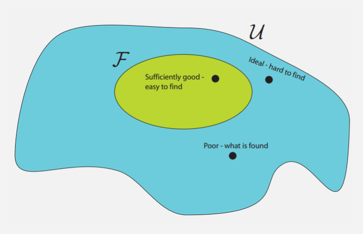
To paraphrase my professor:

Sometimes it’s better to find an exact solution to an approximate problem [exact inference on F] than to find an approximate solution to an exact problem [approximate inference on U].