Part Of: Chess sequence
Followup To: Decision Trees In Chess
Content Summary: 1500 words, 15 min read

Chess Is A Nested Algorithm

In An Introduction To Chess, I introduced you to the basics of chess analysis: how to tell when one position is better than another. Specifically, we looked at material, pawn structure, space, king safety, piece development, piece cohesion, and initiative. These ways of thinking about different chess positions were combined into a score. The first aspect of chess thought lies in the maturation of such an scoring function.

In Decision Trees In Chess, I introduced you to the basics of chess decision making: how to evaluate different alternatives when you are not sure what to do. Specifically, we looked at how imagining different scenarios can be represented in decision trees, how these trees ultimately use scoring functions in their leaf nodes. These decision trees produce decisions after application of the minimax algorithm.

Together, scoring functions and decision trees describe the entirety of what it is to do chess. Had this series been written by world champion Magnus Carlsen, I submit that even he could communicate effectively using this two-part framework. The only things that need be different would be his analysis (his scoring function would be more accurate) and his choice of alternatives to analyze (his considered choices would contain fewer bad alternatives). In other words, skill in chess is not doing more than score functions and decision trees. It is doing them well.

Two Kinds Of Score

Consider the following. White’s turn, can you find mate in two moves?

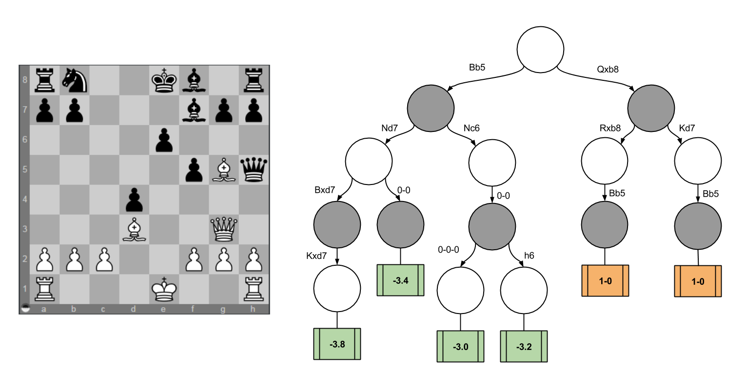
The solution to this puzzle, displayed on the rightmost decision tree, is Qxb8+. If Black recaptures, White checkmates with Bb5# (note that the Bg5 prevents Black’s king from escaping (and if Black runs away Kd7, he is met with the same fate).

Now, imagine if White had not found this clever solution immediately. Suppose White instead tries to attack Black with Bb5+. White’s reflections could lead him to consider the other decision tree, which ultimately values Bb5 as -3.2 points (do you see why the minimax algorithm requires this to be the case?)

Consider the returned values (1-0 WIN) for Qxb8+, and (-3.2) for Bb5. This incongruity is itchy. Why would the scoring function return different types of answers depending on the position?

Meet The SuperTree

Imagine for a moment the decision tree for all chess games. Call this object the SuperTree. What does it look like?

Consider the following facts:

1. On move zero, all chess games ever begin in the same position.
2. After white’s first move, all chess games ever are in one of twenty possible positions (White has 20 legal moves)
3. After Black’s first move, all chess games ever are in one of four hundred possible positions (20*20)
4. All chess games ever conclude with a result (White wins, Black wins, or tie). Some games finish quickly, others take many moves.

These facts can be consolidated into the following visualization:

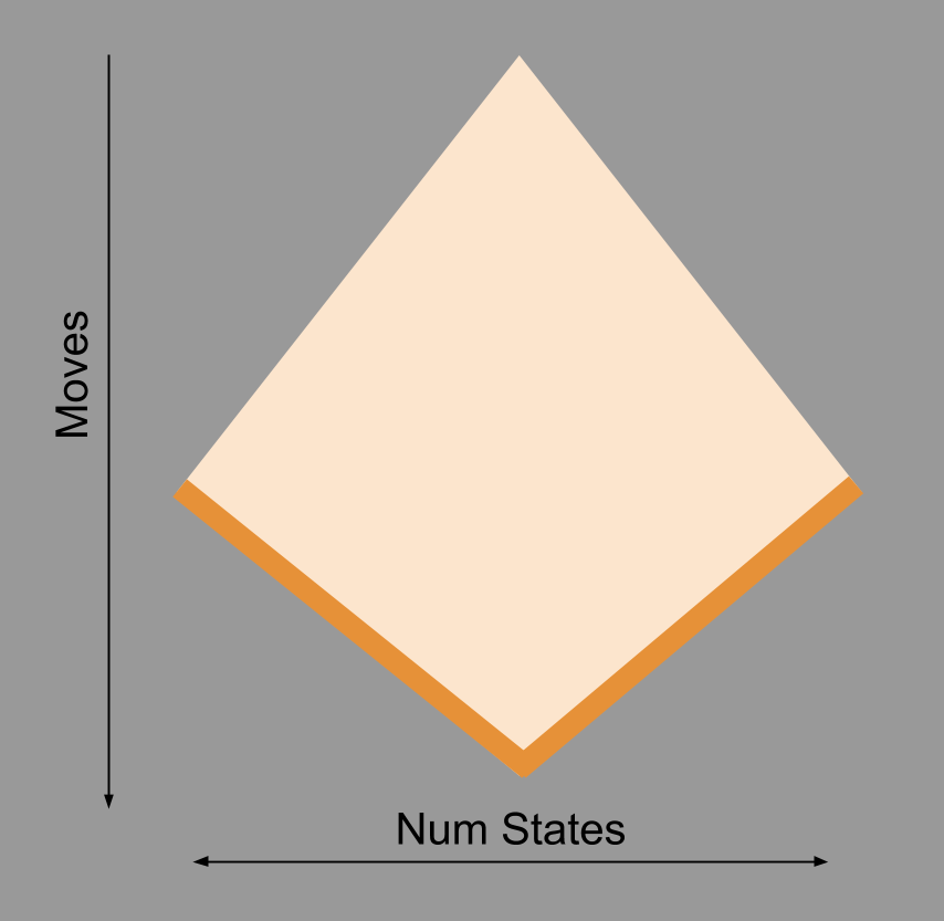
Consider the top of the SuperTree: as we move our gaze downwards, its width increases. This corresponds to our observation above that, as more moves are made, the number of possible positions rapidly increases.

Why then does the number of possible positions decrease as we move into the endgame? Well, you have surely noticed how endgames tend to feature fewer pieces. Consider all chess games that have transitioned into King+Queen vs. King. There are only a few thousand ways to place these three pieces on the board (64*63*62 = 249,984 is an upper bound). Fewer pieces means fewer states (which is why the Supertree is shown as a diamond, not of a triangle).

At the end of every game, at the end of a game tree, are result nodes. This are represented by the dark orange boundary.

We have so far analyzed two game positions: my game from the Decision Trees In Chess post, and the Mate-In-Two position above. Since the above cartoon claims to comprise all chess games that can ever be played, let’s see how these games fit into the SuperTree.

On the left, we see that the Mate-In-Two game line from this post is shorter: this reflects that it (presumably) terminated in the early middlegame, whereas my opponent in the last post survived until the 53rd move.

On the right, we see the decision trees we constructed at moments in each of these games. Pay attention to the coloring of these trees: in the earlier analysis, our endpoints we numerical scores (green) which propagate up to the top of the triangle. In today’s analysis, our endpoints contain a mixture of numerical scores (green) and final results (orange). In this case, by minimax logic, the orange style of result successfully propagated to the top of the decision tree.

Can Chess Be Solved?

Final results, like numerical scores, propagate up a decision tree. If we start at the end of chess games, and work our way backwords, could we color the entire cartoon orange? Could we banish these numerical scores and solve chess? By “solve chess”, I mean be able to prove perfect play; that is, to be able to prove, from any position, the correct move (including move 1).

Lest I be accused of dreaming of something too implausible, precisely this has been done for games like Checkers and Connect-4 (more examples here).

It turns out that chess has been partially solved: computer scientists have managed to solve all games that land in King+Queen vs. King positions. Don’t believe me? Go here, and experience for yourself what it is like to play against God.

We can visualize on our cartoon how computer scientists have managed to “pull orange upwards” in an attempt to solve the SuperTree. These results are typically referred to as tablebases.

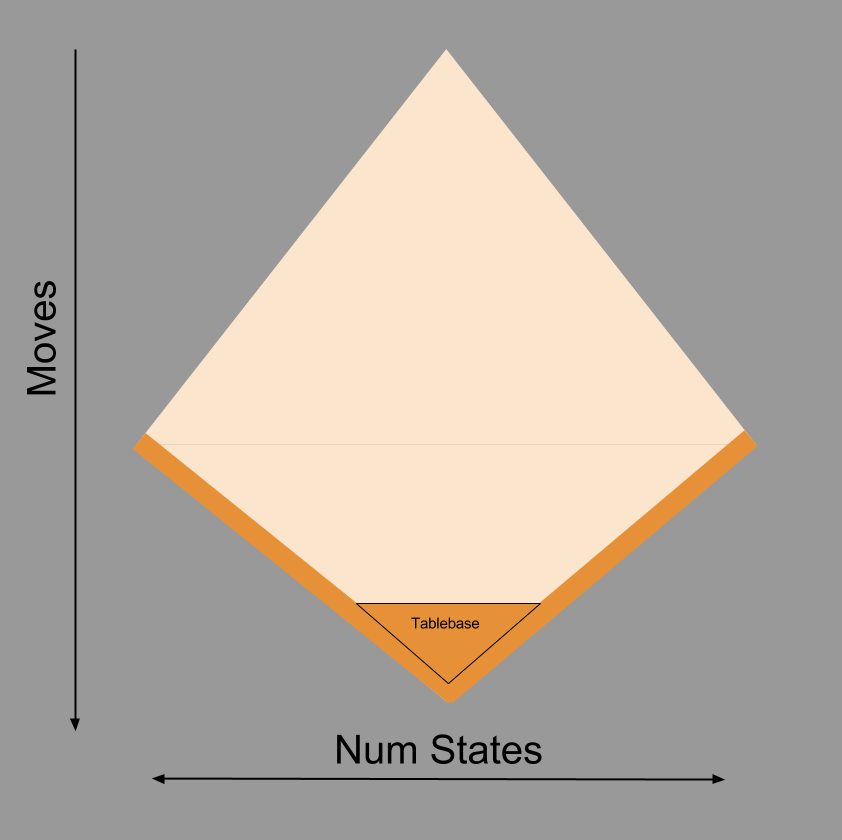
Why haven’t tablebases reached the top of the SuperTree? Compare the size of tablebases as we increase the number of pieces. A three-piece tablebase would include, for example, our classic example of King+Queen vs. King. Such a tablebase only requires 62 kilobytes of memory. But consider what happens when we accomodate more pieces:

To my knowledge, to date our modern supercomputers have failed to construct a complete 8-piece tablebase. Chess begins with 32 pieces. From the table above, when do you think the human race will possess enough computing resources to implement a 32-piece tablebase? 🙂

A Role For Numeric Scores

We now see why our scoring function cannot return game results for most moves in our path.

Consider the case where the results of the Supertree propagate upwards in a completely unpredictable manner. In this situation, we could do no better than rolling a dice to make our move, because no move can increase or chances of winning (or losing, or drawing).

But chess is not like this. Suppose you convince two evenly-matched players to play 100 games, and you remove the queen from the first player’s starting position before each match begins. The second player will probably win many more than 50 games. This tells us that chess results are not completely unpredictable. Locations in the SuperTree in which one player has a material advantage have an above-average chance of leading to a Win result, just as material disadvantages tend to balance the scale towards the Lose result. Given this window of improved predictability, we can prefer moves that improve our material situation.

Most moves in chess, regrettably, do not yield a material advantage. Can we do better than rolling the dice? Do there exist materially-equal positions where, when given to evenly-matched players, one player will win more frequently? Of course there are. We met some of these measures in An Introduction To Chess, for example:

• Pawn structure. Some pawn configurations are more stable and defensible than others.
• Space. Some pawn configurations allow a player relatively more room to maneuver.
• King safety. How many defensive resources does a player have near his King?
• Piece development. At what rate has one managed to bring pieces into the fight?
• Piece cohesion. Are one’s pieces working together well?
• Initiative. Who is making more threats, and dictating the course of the game?

Skill in chess is nothing more, and nothing less, than this: the ability to discover new features (patterns in the Supertree) and the ability to “mix & match” all features to produce a single move recommendation.

This is why our “green” numeric results are are so vital. Despite not knowing the true state of the underlying SuperTree, iteratively maturing your score function provides a player with an increasingly confident prediction of the SuperTree’s true value. In other words, these aggregations of different features comprise a heuristic flashlight that gives clues about the SuperTree.

Takeaways

• Chess decisions are made via a nested algorithm.
  • At the higher level, a player must compute a decision tree, and make decisions by rolling up the leaf scores via the minimax procedure.
  • At the lower level, for each node in the decision tree, a player must invoke a scoring function to evaluate the desirability of that position.
• Some decision trees can be evaluated as Win/Lose/Draw, rather than a particular number.
• The SuperTree – the decision tree that contains all possible moves of any possible game – is a useful way to think about the game of chess.
• We can think of specific games as traces in the supertree, and understand why attempts to solve the SuperTree (tablebases) have proved intractable.
• Scoring functions only work if they provide access to regularities within the underlying SuperTree.