The Fundamental Theorems of Evolution

October 27, 2026October 27, 2026kevinbinz Leave a comment

Part Of: Biology sequence
Followup To: Intro to Replicator Dynamics
Content Summary: 7000 words, 35 min read

Introduction

In 1977, a drought struck Daphne Major, a small island in the Galápagos. Most ground finches died. The survivors could crack the hard seeds that remained, and their beaks averaged about half a millimeter deeper than the population’s before the drought. If the survivors had deeper beaks, we might expect their offspring to express these characteristics. But how much of the survivors’ shift will their chicks inherit?

The replicator equation cannot answer. That formalism requires a list of variants whose members have the same kinds of offspring. But finches with the same beak depth don’t all have the same chicks.

To predict what happens to the chicks, we require a new formalism without these limitations. This post develops the Price equation, which allows us to tease apart selection and transmission.

Let’s dive in!

The Fundamental Theorem of Evolution

The replicator–mutator equation tracks a list of variants. Selection multiplies the count of each variant by its fitness through the fitness matrix W. Heredity (Q), the process by which offspring resemble their parents, moves offspring into variants:

$n^{\prime} = QWn$

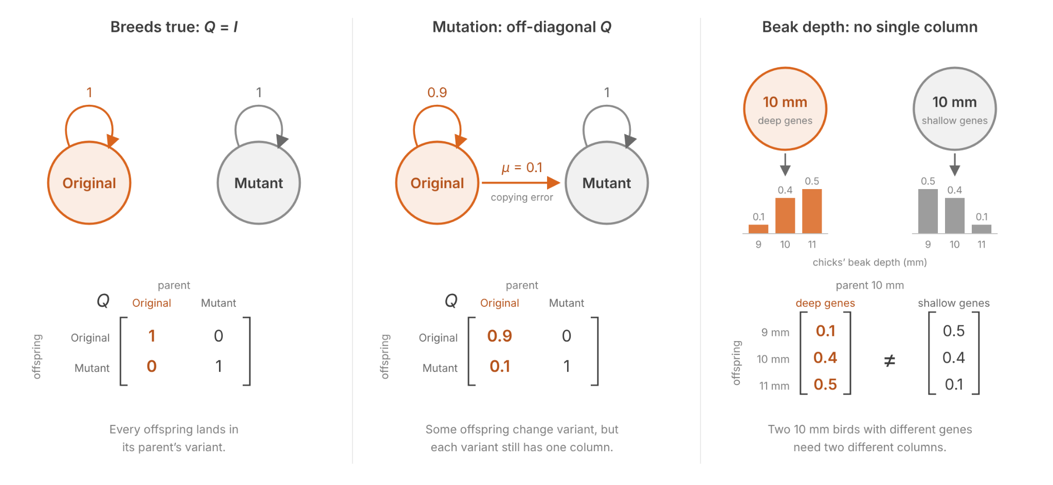
A variant is a class of individuals that meets three requirements:

Same fitness: one entry of W per variant.
Same kinds of offspring: one column of Q per variant.
Breeds true: that column is the identity’s.

Mutation relaxes the third condition by letting Q be nonzero off the diagonal, hence its usual name, the mutation matrix. But finches grouped by beak depth break the second condition. Finches with the same beak depth don’t all produce the same kind of offspring. Two finches with 10 mm beaks can carry different genes, and so have different chicks.

But we can still reason about the average beak depth, and how it changes. Consider finches grouped by their beak depths. Let’s imagine a particular class i with beak depths between 10.0 and 10.1 mm. Then:

$xᵢ$ is the class frequency: the number of birds in the class, divided by the population size.
$wᵢ$ is its average number of offspring.
$zᵢ$ is its average beak depth (e.g., about 10.05 mm).
$\textstyle \varDelta z_i$ is the change from $zᵢ$ to their offspring’s average beak depth.

Next, count the offspring by their parent’s class, not their own. Let $xᵢ′$ be the fraction of chicks that descend from class i, and $zᵢ′$ the mean beak depth of those chicks. The change in mean beak depth is:

$\displaystyle \varDelta\bar{z} = \bar{z}^{\prime}-\bar{z} = \sum_i x_i^{\prime} z_i^{\prime}-\sum_i x_i z_i$

We also let $z̄*$ be the parents’ mean beak depth, with each parent counted once per chick:

$\bar{z}^{*} = \sum_i x_i^{\prime}\,z_i$

Mean fitness w̄ is the average number of offspring per parent, and wᵢ/w̄ is the class’s relative fitness. Then:

$xᵢ′ = xᵢwᵢ/w̄$ multiplies class frequency by relative fitness.
$\textstyle z_i^{\prime} = z_i + \varDelta z_i$ ᵢ adds the chicks’ shift to their parents’ mean.

The change in mean beak depth can be expressed as two differences.

$\displaystyle \varDelta\bar{z} = (\bar{z}^{*}-\bar{z}) + (\bar{z}^{\prime}-\bar{z}^{*})$

In the first step, parent classes that leave more chicks pull the mean toward their beak depth. Appendix A shows that the shift is set by the covariance of fitness and trait:

$\bar{z}^{*}-\bar{z} = \frac{\operatorname{Cov}(w,z)}{\bar{w}}$

In the second step, the chicks of class i sit Δzᵢ from their parents’ mean. Averaged over all chicks, the second step is (Appendix A):

$\displaystyle \bar{z}^{\prime}-\bar{z}^{*} = \frac{\operatorname{E}(w \varDelta z)}{\bar{w}}$

Add the two steps. The result is the Price equation (Price 1970):

$\displaystyle \varDelta\bar{z} = \frac{\operatorname{Cov}(w,z)}{\bar{w}} + \frac{\operatorname{E}(w \varDelta z)}{\bar{w}}$

The Price equation has two terms:

The first term is the selection differential S: the change selection alone would make if every offspring were a copy of its parent. It comes from the first step, which for listed variants comes from the fitness matrix W.
The second term is the transmission T: how far offspring differ from their own parents, averaged over all offspring. It comes from the second step, which for listed variants comes from the mutation matrix Q. Other sources write T out in full; the letter is this post’s.
R, the response to selection, is another name for the left side, Δz̄. The name assumes that selection moved the mean, though T can move it with no selection at all, for example through mutation bias or a change in environment.

Another way to express the Price equation, then, is:

$R = S + T$

Classically, selection is split into three episodes: survival to breeding age, mating success, and fecundity (Arnold & Wade 1984). Our drought data cover only survival, so we assume that survival is all of selection. In other words, survivors of every beak depth raise the same number of chicks on average, a constant c:

$\operatorname{E}(\text{chicks} \mid \text{survived}, z) = c$

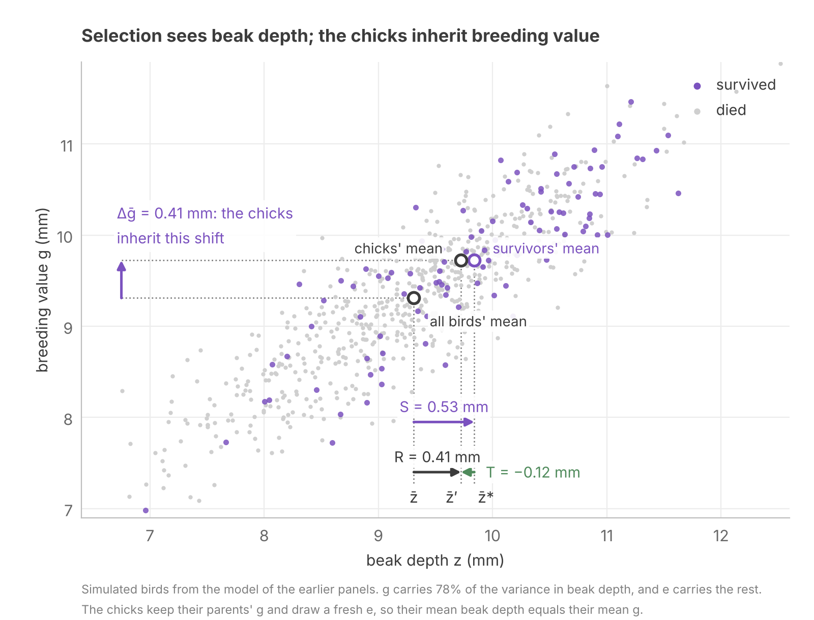
With this assumption, $xᵢ′$ is the fraction of survivors in class i. So $z̄*$ , the mean after selection, is the survivors’ mean. The figure puts the drought’s means on a number line, using the chicks’ mean that a later section predicts:

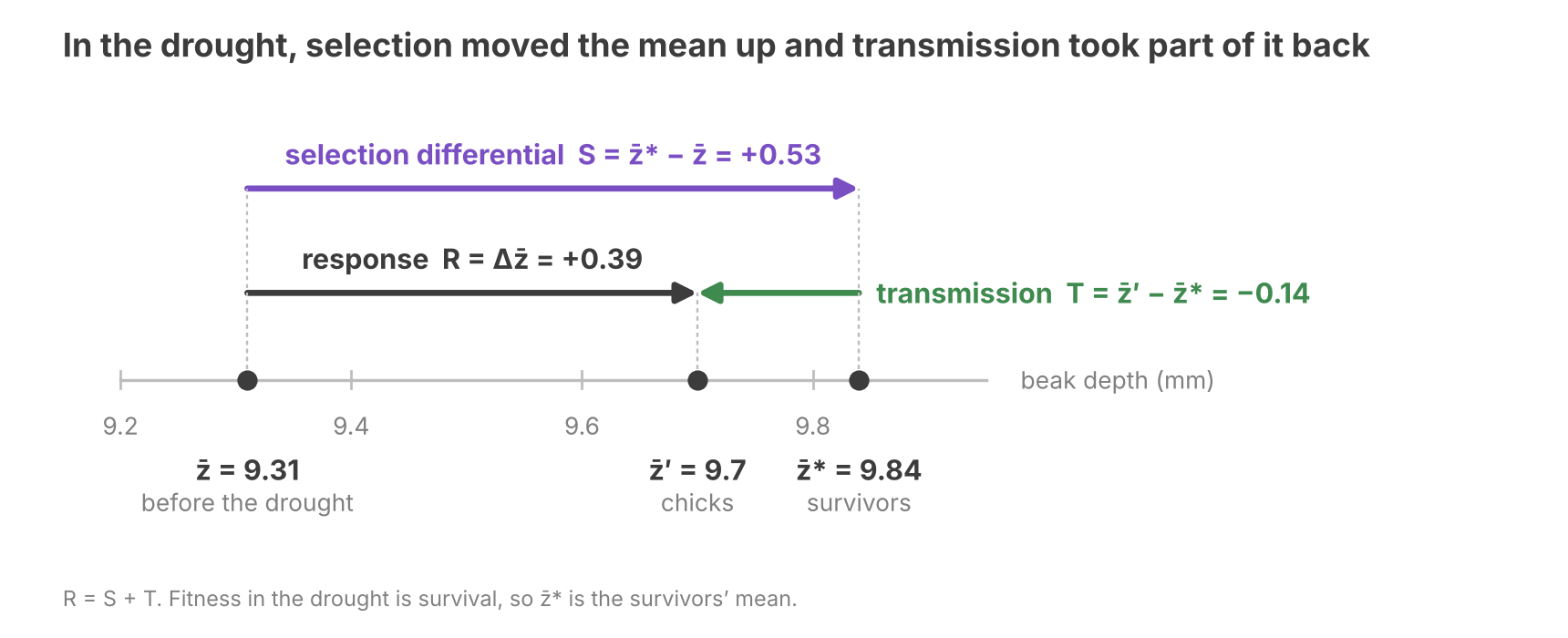
The Price equation holds for any trait and any rule of inheritance. Changing bin size doesn’t change R, only the balance between S and T.

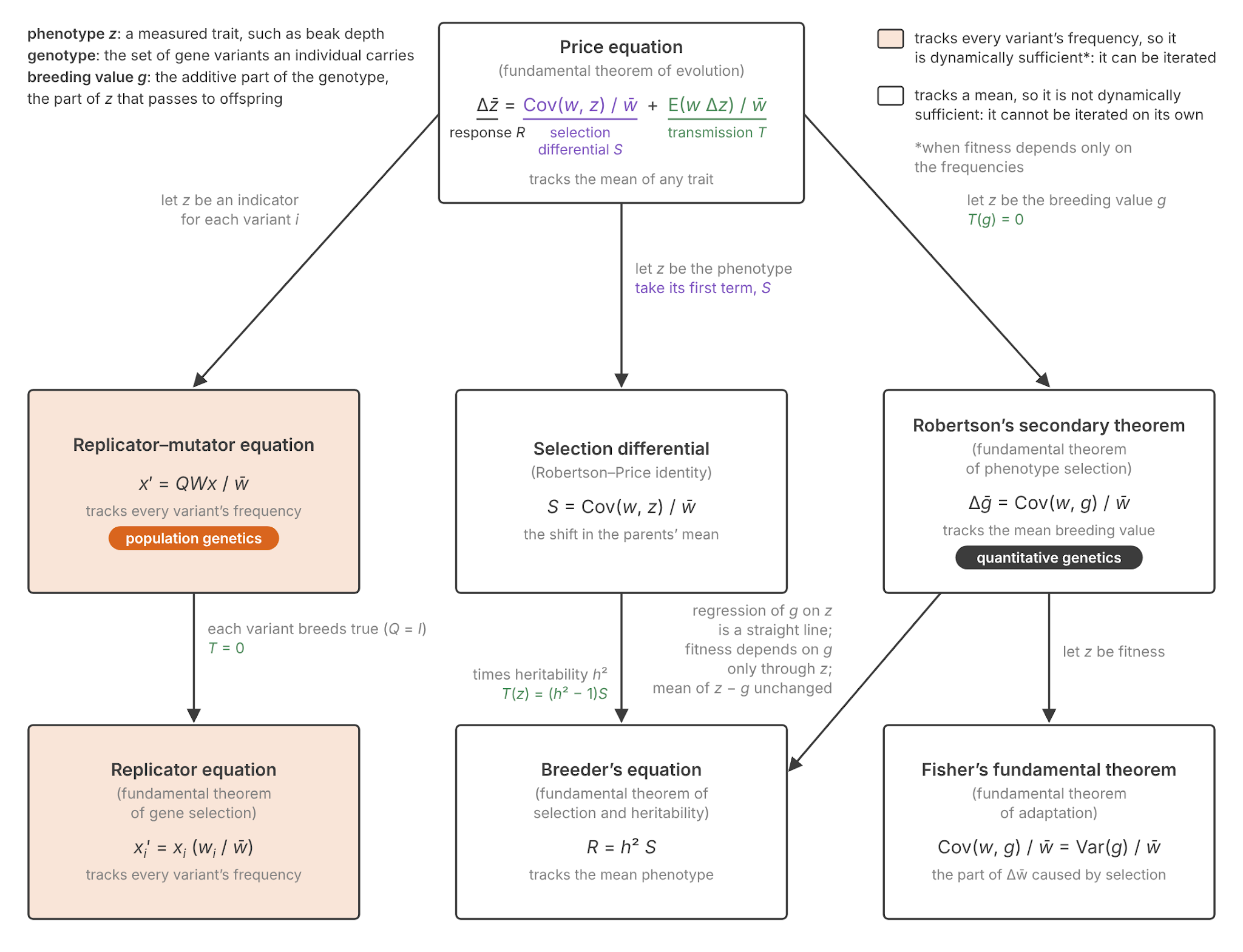
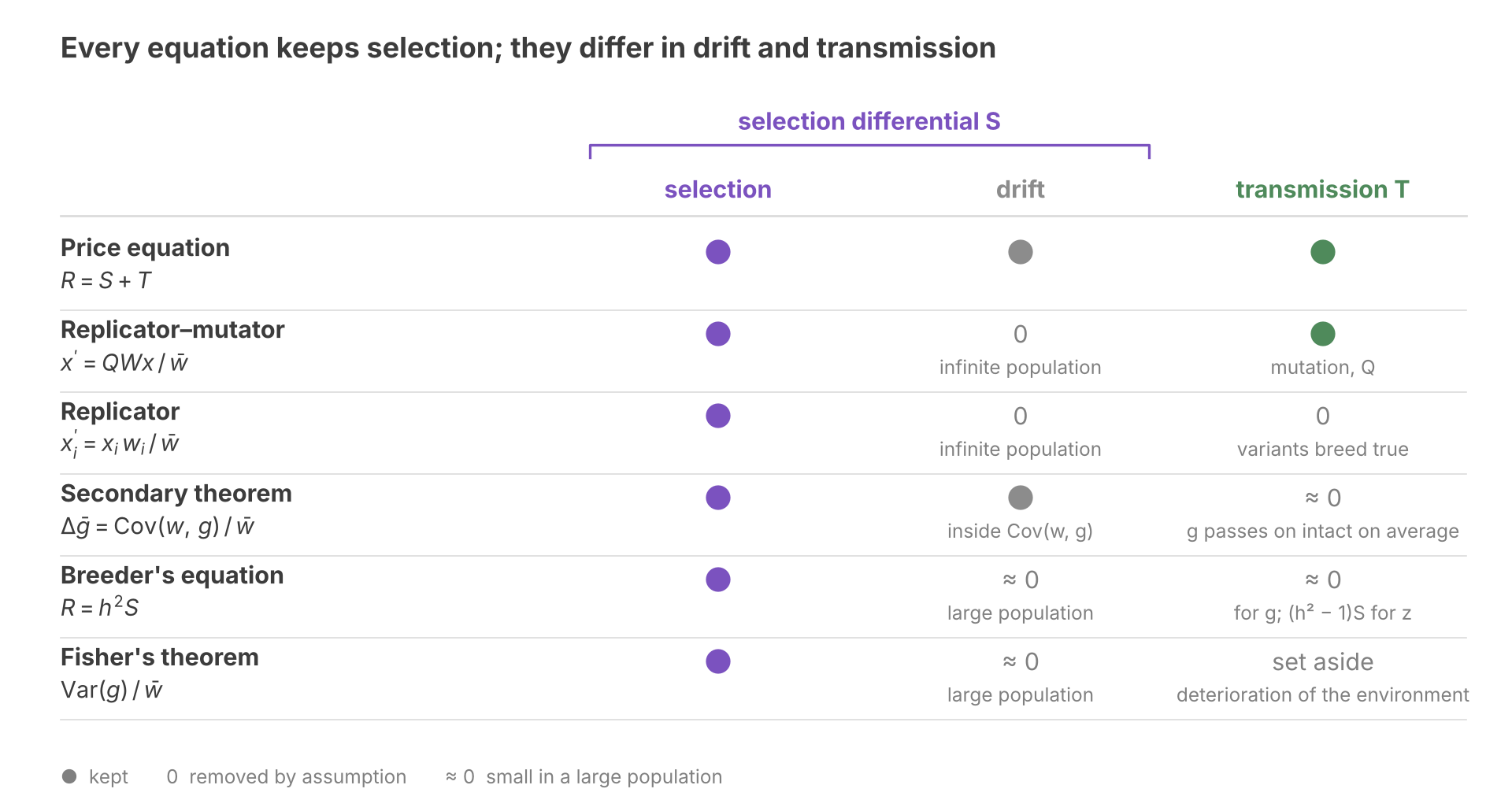
The Price equation is described by Queller (2017) as the fundamental theorem of evolution. It sits at the top of a family of classical results, bridging the gap between methods in population genetics and quantitative genetics. The following tree is adapted from his, and our section titles use his names.

The Theorem of Gene Selection

This section derives the replicator equation from the Price equation, following the left branch of the tree.

Let z be an indicator variable: 1 for variant i, and 0 for other variants. The mean of an indicator variable is its frequency:

$\bar{z} = x_i$

The left side of the Price equation becomes:

$\displaystyle \varDelta\bar{z} = \bar{z}^{\prime}-\bar{z} = x_i^{\prime}-x_i = \varDelta x_i$

Substitute the indicator into S. Only variant i has z = 1, so only its fitness enters the covariance (Appendix B):

$\frac{\operatorname{Cov}(w,z)}{\bar{w}} = x_i\,\frac{w_i-\bar{w}}{\bar{w}}$

This is the replicator equation’s change in frequency: what selection does when every offspring copies its parent.

An offspring of a variant-k parent lands in variant i with probability $\textstyle Q_{ik}$ . That probability is the mean z of its offspring, so the change in z for a variant-k parent is:

$\displaystyle \varDelta z_k = Q_{ik}-z_k$

For variant i, T measures the balance of mutation inflow and outflow:

$\displaystyle \frac{\operatorname{E}(w \varDelta z)}{\bar{w}} = \text{inflow}-\text{outflow} = \frac{\sum_{k\neq i} Q_{ik} w_k x_k}{\bar{w}}-\frac{(1-Q_{ii}) w_i x_i}{\bar{w}}$

Add S and T to $xᵢ$ . Every term cancels except the flow through Q (Appendix B):

$x_i^{\prime} = \frac{\sum_k Q_{ik}\,w_k\,x_k}{\bar{w}}$

In matrix form, with W the diagonal matrix of fitnesses, this is the replicator–mutator equation in frequencies:

$x^{\prime} = \frac{QWx}{\bar{w}}$

If each variant breeds true, Q is the identity matrix and T vanishes. The sum for $xᵢ′$ then keeps only its k = i term, which is the replicator equation:

$x_i^{\prime} = x_i\,(w_i/\bar{w})$

The three equations form a ladder, each rung more general than the one below:

The replicator equation tracks the frequency of every variant and assumes each variant breeds true.
The replicator–mutator equation also tracks every frequency, and lets copying errors move offspring between listed variants.
The Price equation tracks the mean of any trait, and allows any rule of inheritance.

We now turn our attention to quantitative genetics. All of its equations require an extra assumption to predict past one generation. The Moment Hierarchy section explains why.

The Selection Differential

Let’s reconsider how drought affected beak depth:

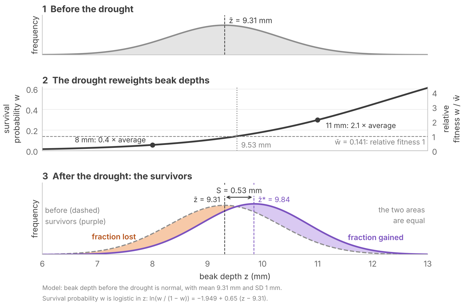
Recall that the selection differential S is the shift in means before and after selection:

$S = \bar{z}^{*}-\bar{z}$

In the drought, the mean rose from 9.31 mm to 9.84 mm among the survivors (Grant 1986), so S is 0.53 mm.

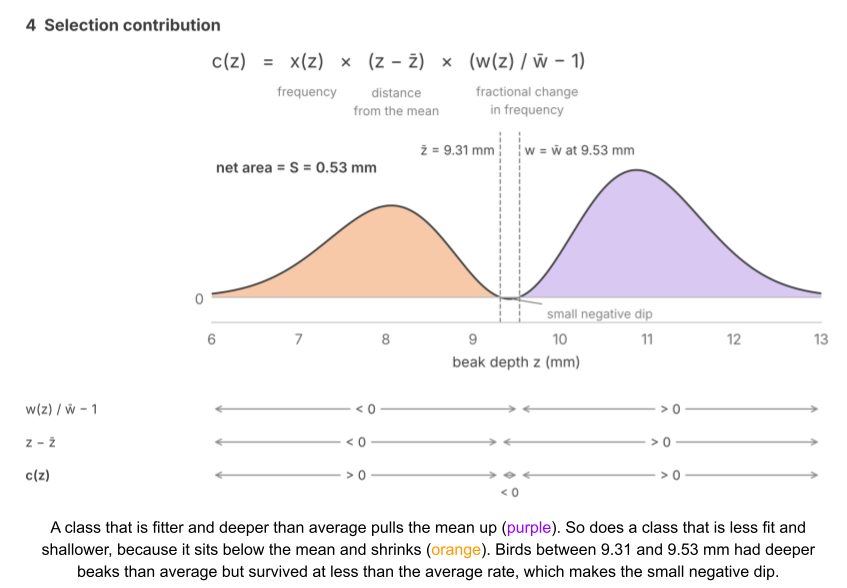
Written out, S sums the product of two deviations, weighted by class frequency xᵢ:

$\displaystyle S = \sum_i x_i\left(\frac{w_i}{\bar{w}}-1\right)(z_i-\bar{z}) = \frac{\operatorname{Cov}(w, z)}{\bar{w}}$

$wᵢ/w̄ − 1$ sets how much its fraction changed.
$zᵢ − z̄$ sets how far from the mean that fraction sits.

Covariance measures net alignment between these deviations. When matching signs dominate, selection raises the mean. When opposite signs dominate, selection lowers it.

Biologists measure S in the field the way the Grants did. They measure a trait across individuals, while also recording who survives or reproduces. Over 2,500 estimates of selection from 63 studies show that most selection in nature is weaker than in the drought (Kingsolver et al 2001). Breeders instead impose S, by choosing which animals breed.

S mixes two causes of differential reproduction: trait and luck. To separate them, imagine replaying the drought many times with the same birds. Let expected fitness $f(z)$ be the average fitness of birds with beak depth z over the replays. A bird’s fitness w is what it actually had in this one drought. It differs from expected fitness by ε, the part of its fitness that beak depth does not explain:

$w = f(z) + \varepsilon$

Averaged over the replays, ε is zero at every beak depth:

$\operatorname{E}(\varepsilon \mid z) = 0$

So ε has no covariance with beak depth on average, but in any one drought luck makes it covary by chance. Taken together, we have decomposed S into two terms.

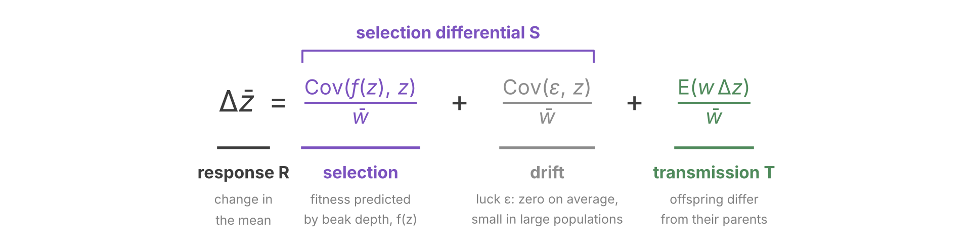
The rest of this post will assume a large population, where drift is small.

The Breeding Value

S is a shift in the parents, and the population evolves only if the offspring shift too. But heredity passes on genes, not beak depth. A bird’s beak depth also depends on its conditions as a chick, such as the food it received, and that part usually doesn’t pass on. So the offspring keep only part of S. To find how S is carried across generations, we need to decompose z.

A phenotype (z) is a measured trait, such as beak depth. An individual’s breeding value (g) is the part of its phenotype that its offspring inherit on average. Call the rest u:

$z = g + u$

What g contains depends on how the species reproduces. A genotype is the set of gene variants an individual carries, and its genotypic value (G) is the average phenotype of individuals that carry it.

In clonal reproduction, the whole genotype passes intact to the offspring, so the breeding value is the genotypic value and the rest is environmental deviation (e):

$g = G, \quad u = e$

But in sexual reproduction only part of G passes. A parent passes along only one allele per locus.

Imagine a locus with two equally prevalent alleles B and b. BB, Bb and bb birds have beaks 9.4, 9.4 and 9.0 mm deep, respectively. With random mating, Bb birds are twice as common as BB or bb birds, so the population mean is:

$\bar{z} = \tfrac{1}{4}(9.4) + \tfrac{1}{2}(9.4) + \tfrac{1}{4}(9.0) = 9.3\text{ mm}$

A chick gets one allele from each parent, so its second allele is B or b with equal odds. Chicks that get B average 9.4 mm whatever their second allele, and chicks that get b average 9.2 mm, halfway between 9.4 and 9.0. Measured from 9.3, that is +0.1 and −0.1 mm. Adding a bird’s two allele effects to the population mean gives its breeding value. And indeed, offspring of a Bb finch average 9.3 mm, not 9.4 mm. Dominance (D) is the remainder: genotypic value minus breeding value. It denotes the interaction between the two alleles at one locus.

Genotype	Genotypic value (G)	Breeding value (g)	Dominance (D)
bb	9.0 mm	9.1 mm	−0.1 mm
Bb	9.4 mm	9.3 mm	+0.1 mm
BB	9.4 mm	9.5 mm	−0.1 mm

Interactions between alleles at different loci, epistasis (I), are mostly broken up the same way when meiosis reshuffles alleles across loci.

In a sexual species, then, the genotypic value has three parts:

$G = g + D + I$

Substitute it into the phenotype:

$z = (g + D + I) + e$

With minor exceptions, a parent passes on its g but not its D or I, so for transmission D and I behave like e. So the rest u holds all three:

$u = D + I + e$

The Theorem of Phenotype Selection

Recall that beak depth splits into its breeding value g and the rest u:

$z = g + u$

To apply the Price equation to all three variables, we write the trait as an argument. For any trait y:

$R(y) = S(y) + T(y)$

$\displaystyle S(y) = \frac{\operatorname{Cov}(w,y)}{\bar{w}}, \quad T(y) = \frac{\operatorname{E}(w \varDelta y)}{\bar{w}}, \quad R(y) = \varDelta\bar{y}$

Without an argument, S, T and R refer to z.

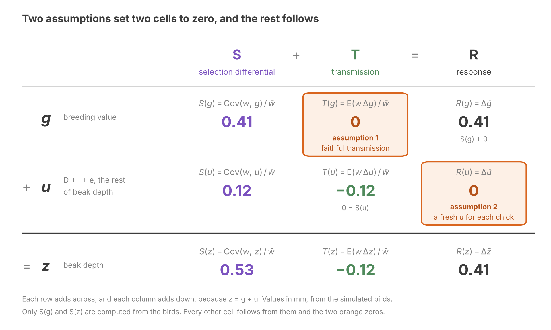
We begin with one assumption, faithful transmission: the chicks’ mean g equals the mean g of their parents, so T(g) vanishes. In a sexual species, faithful transmission also requires fair meiosis: each allele must have an equal chance of reaching a chick. Mutation and meiotic drive break these assumptions, respectively.

$\displaystyle T(g) = \frac{\operatorname{E}(w \varDelta g)}{\bar{w}} = 0$

Apply the Price equation to g. Faithful transmission removes T(g):

$\Delta\bar{g} = \frac{\operatorname{Cov}(w,g)}{\bar{w}}$

That is:

$R(g) = S(g)$

This is Robertson’s secondary theorem of natural selection (Robertson 1966; Price 1970). Like the Price equation, this theorem generalizes to any heritable state, not just nucleic acids. It applies for any state that offspring receive faithfully, such as the song a male finch learns from its father (Grant & Grant 1996).

But g is a latent variable. To model how observable z changes, we need a second assumption. We assume parents only pass down g, and nothing else that shapes the trait, and that the environment stays the same. Then each chick draws a fresh e, and meiosis gives it fresh D and I. Then R(u) vanishes.

$\displaystyle R(u) = \varDelta\bar{u} = 0$

Applying Price on u:

$0 = S(u) + T(u)$

Selection sorts the finches by z, but the chicks inherit g. Some survivors had deep beaks due to environmental factors, so the survivors’ mean g moved less.

Splitting z splits the covariance:

$\operatorname{Cov}(w,z) = \operatorname{Cov}(w,g) + \operatorname{Cov}(w,u)$

Divide both sides by w̄:

$S(z) = S(g) + S(u)$

S(g) is the shift the chicks inherit, and the environmental covariance S(u) is the part they do not. Note that u can hold dominance and epistasis, which are genetic but are broken up by meiosis.

On the Isle of Rum, red deer with heavier antlers have more offspring. Yet over nearly 30 years, the average antler size did not increase, despite the trait being heritable (Kruuk et al 2002). The authors proposed a nutrition confound: a well-fed stag grows heavy antlers and also wins more contests for mates. Nutrition contributes to S(u), which explains nearly all of S.

We have applied the Price equation to three variables. We can visualize this as a table, and our assumptions correspond to zeroed cells. Every other cell follows.

The rest of this post builds on Robertson’s theorem. Breeding values cannot be observed directly, so The Breeder’s Equation estimates this covariance from traits we can measure. Fisher’s fundamental theorem takes fitness itself as the trait.

The Breeder’s Equation

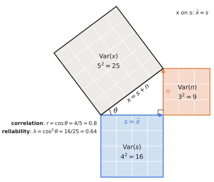
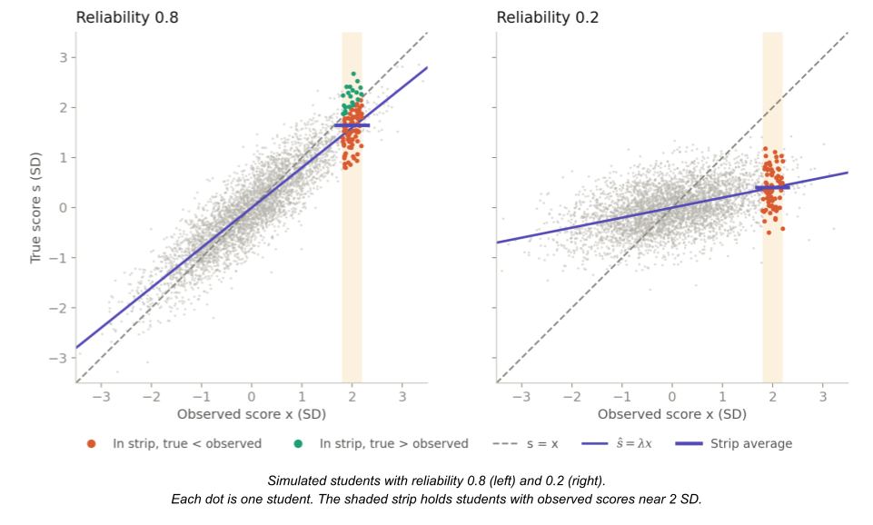
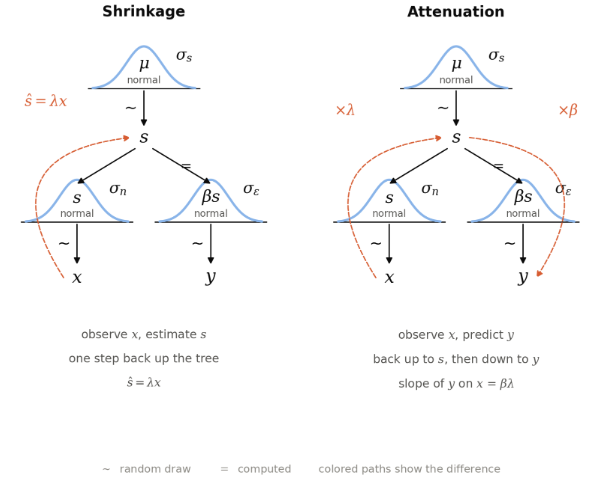
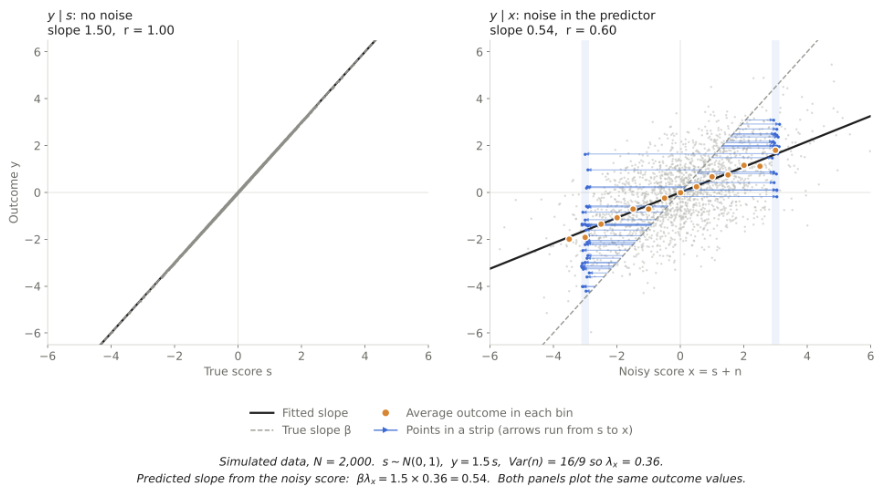
Heredity carries g, so a phenotype is a noisy measurement of the part that passes on. The results of The Reliability Ratio carry over directly:

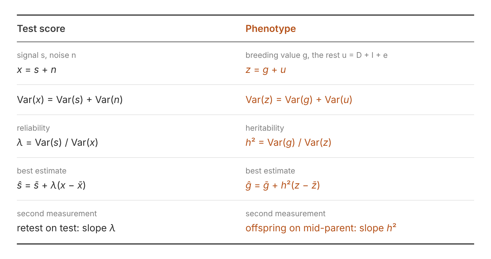
The estimate starts from a regression. When u is independent of g, the slope of the regression g on z is the reliability:

$\frac{\operatorname{Cov}(g,z)}{\operatorname{Var}(z)} = \frac{\operatorname{Var}(g)}{\operatorname{Var}(z)} = h^2$

Here, we call the reliability the narrow-sense heritability (h²), the fraction of the variance in beak depth that comes from breeding values.

To derive the breeder’s equation, we need Kelley’s rule from The Reliability Ratio. That requires two assumptions. First, u is independent of g, as the slope above assumed. Second, g and u are normally distributed. Kelley’s rule then puts the average g at each beak depth on the regression line:

$\operatorname{E}(g \mid z) = \bar{g} + h^2\,(z-\bar{z})$

Here we need one more assumption: fitness depends on g only through z.

$\operatorname{E}(w \mid z, g) = \operatorname{E}(w \mid z)$

Fitness sees only z, so it sees g only through the average g at each beak depth, and Kelley’s rule shrinks that average toward the mean by h². Appendix C works through the steps. The result converts Robertson’s covariance into one we can measure:

$\operatorname{Cov}(w,g) = h^2\,\operatorname{Cov}(w,z)$

Divide both sides by w̄, and apply Robertson’s theorem:

$R(g) = S(g) = h^2 S$

Recall that $z = g + u$ . This splits the response to selection:

$R = R(g) + R(u) = h^2 S + R(u)$

The second assumption of The Theorem of Phenotype Selection removes the last term:

$R = h^2 S$

This is the breeder’s equation. It splits Robertson’s covariance into two factors, S for selection and h² for the fraction of S that passes on, so that each can be measured on its own.

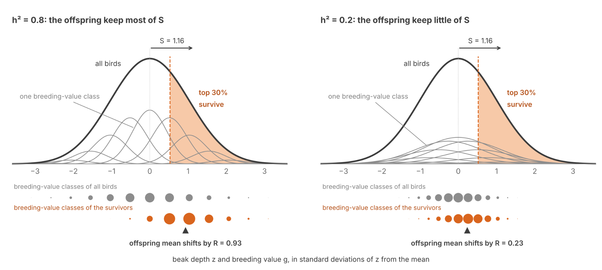
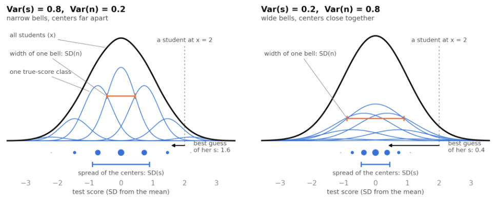
The figure shows how heritability sets the response. Each gray curve is one breeding-value class, and the black curve is the whole population, with beak depth in standard deviations. Both panels have the same population curve, and the same selection pressures, so S is the same. The survivors differ. On the left, the classes are narrow, and the survivors come mostly from classes far to the right. On the right, the classes are wide, and the survivors come mostly from classes near the middle. The offspring inherit their parents’ breeding values, so R is 0.93 SD on the left and 0.23 SD on the right.

For the finches, Boag (1983) measured a heritability of 0.78 for beak depth. The breeder’s equation predicts the response in the offspring of the survivors:

$R = 0.78\times 0.53\text{ mm} = 0.41\text{ mm}$

That predicts a mean of 9.72 mm for the chicks.

Recall that T = R − S. Now, substitute the breeder’s equation and factor:

$T = h^2 S-S = (h^2-1)\,S$

For beak depth:

$T = (0.78-1)\times 0.53\text{ mm} \approx -0.12\text{ mm}$

$0.41 \approx 0.53 + (-0.12)$

The 0.12 mm that does not pass on is T for beak depth. The breeder’s equation predicts that the chicks of deep-beaked survivors fall back toward the mean. This is regression to the mean. Tracked through g instead, the whole response is S(g) and T(g) vanishes.

Heredity, heritability and transmission are easy to conflate.

Heredity (Q) is an individual process across generations. It denotes what each child inherits from its parents.
Heritability (h²) is a population statistic within a generation. It denotes what fraction of trait variance comes from the breeding value. It describes how individuals differ.
Transmission (T) is a population statistic across generations. It denotes change in the mean between selected parents and their offspring. It collects mutation, and everything else that separates children from their parents. Only on the breeder’s assumptions does h² fix T for a given S.

Neither h² nor S alone produces R. If h² = 0, selection acts on the parents but cannot affect the children. If S = 0, heritable state can be copied faithfully, yet selection does not move the mean. Schulman et al (2012) built DNA tiles with high copying fidelity, but every pattern grew at the same rate.

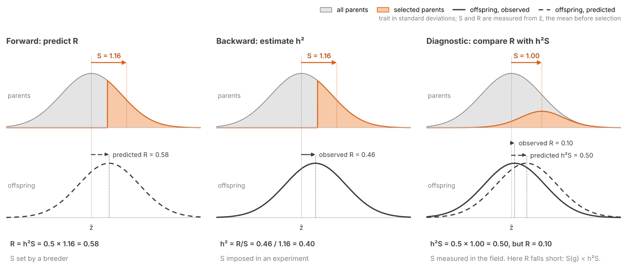
The breeder’s equation can be applied in three ways: forward, backward and diagnostic.

First, if h² and S are known, breeders can forecast R. They use this method to plan their selection process. Conservation biologists calculate whether a population will keep pace with a changing environment.

Second, a selection experiment controls the value of S and measures the resultant response R. Heritability is learned by taking their ratio.

Third, biologists can predict R from the model, and then compare it with the observed R. Prediction errors suggest an assumption mismatch. Here are two cases which challenge the assumption that fitness depends on g only through z.

Heritable traits under strong directional selection often change less than predicted (Merilä et al 2001). The red deer on Rum are one such case. Nutrition drives both antler size and fitness. When fitness depends on the environment directly, S(g) is smaller than the breeder’s equation predicts. In other words, S(g) < h²S.
Grant & Grant (1995) measured both drought generations. Mean beak depth rose from 9.21 mm before the drought to 9.70 mm in the chicks hatched in 1978. In contrast with the breeder’s prediction, the chicks kept nearly all of the survivors’ shift. Why? Well, the drought also favored larger bodies, and birds that inherit larger bodies tend to inherit deeper beaks. When selection also acts on a second trait whose breeding value covaries with g, S(g) can exceed the prediction. In other words, S(g) > h²S.

The forward and diagnostic uses require knowing h². How do we measure it?

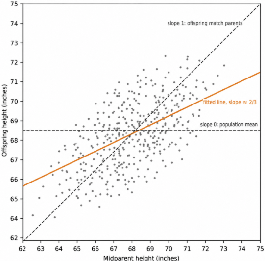
Galton (1886) invented regression to study heredity. Plot each offspring’s trait against the average of its parents, the mid-parent, and fit a line. If offspring were identical to their parents, the line would have slope 1. If chicks inherited nothing from their parents, the slope would be 0. For finch beak depth, the slope is 0.78.

Regression to the mean occurs because offspring play the role of the retest. On average, a chick inherits the g of its mid-parent, but it draws a fresh u. So the slope is the heritability h² (i.e., reliability).

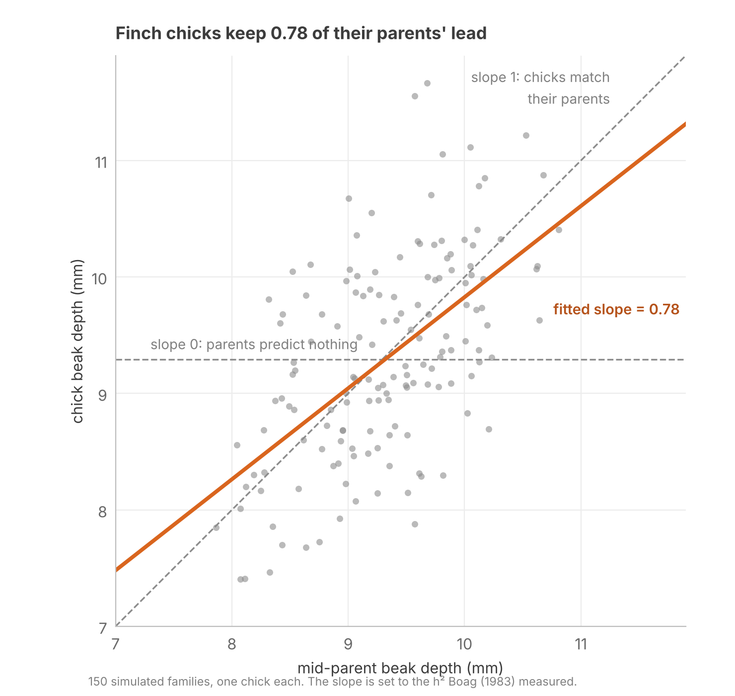
This conclusion only holds when its assumptions are met. The second assumption of The Theorem of Phenotype Selection fails if parents pass along non-genetic components (e.g., territory). In that situation, the slope measures breeding values and inherited environment together.

Fisher’s Fundamental Theorem

Selection improves organisms. Fisher sought to quantify the speed of improvement. He compared his result to the second law of thermodynamics: each law names a quantity that moves only one way.

Choose fitness itself as the trait. Setting z = w in the Price equation gives

$\displaystyle \varDelta\bar{w} = \frac{\operatorname{Var}(w)}{\bar{w}} + \frac{\operatorname{E}(w \varDelta w)}{\bar{w}}$

$R(w) = S(w) + T(w)$

Split fitness like any other trait: w = g + u. Recall the definition of S(g), but substitute g+u into the covariance:

$S(g) = \frac{\operatorname{Cov}(w,g)}{\bar{w}} = \frac{\operatorname{Cov}(g+u,\,g)}{\bar{w}}$

The covariance splits in two, and the covariance of g with itself is its variance. u is uncorrelated with g, so the last term is zero:

$S(g) = \frac{\operatorname{Cov}(g,g) + \operatorname{Cov}(u,\,g)}{\bar{w}} = \frac{\operatorname{Var}(g) + 0}{\bar{w}}$

Applying Robertson’s secondary theorem yields the change in mean fitness caused by selection:

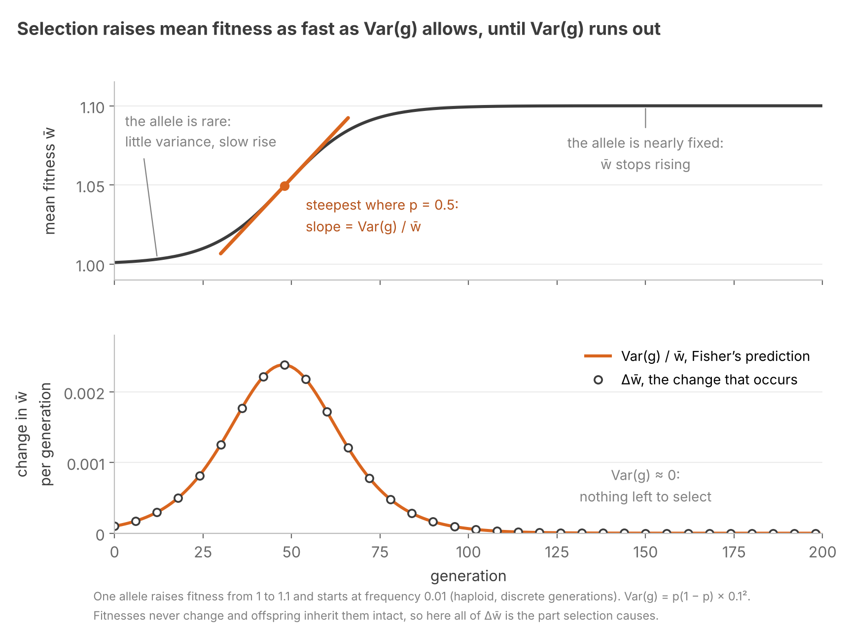
$R(g) = S(g) = \frac{\operatorname{Var}(g)}{\bar{w}}$

This is Fisher’s (1930) fundamental theorem of natural selection. The rate of increase of fitness depends on Var(g), known as the additive genetic variance.

Dividing by w̄ once more gives the fraction by which selection raises mean fitness each generation: $Var(g)/w̄²$ . Houle (1992) called this measure evolvability, a scale on which traits and species can be compared.

Only 15% of the finches on Daphne Major survived the 1977 drought, so the variance in relative fitness was enormous:

$\operatorname{Var}(w)/\bar{w}^{2} = 0.85/0.15 \approx 5.7$

But only its heritable part, Var(g), moved the next generation. If survival had been truly random, the population would not have changed.

Selection runs on heritable variance in fitness. If you measure it, you can predict how quickly selection will proceed. Recall that selection also uses up its fuel. An allele that raises fitness approaches fixation, and a fixed allele adds nothing to Var(g).

Selection tends to drain Var(g) faster than Var(D). Let’s name the dominance ratio:

$\text{dominance ratio} = \frac{\operatorname{Var}(D)}{\operatorname{Var}(g)}$

Harmful recessive alleles increase the dominance ratio. In heterozygotes they are masked by dominant alleles. Selection sees them only in the rare homozygotes, so they linger, and most of the variance they cause is Var(D). Inbreeding exposes these hidden recessives by making them homozygous.

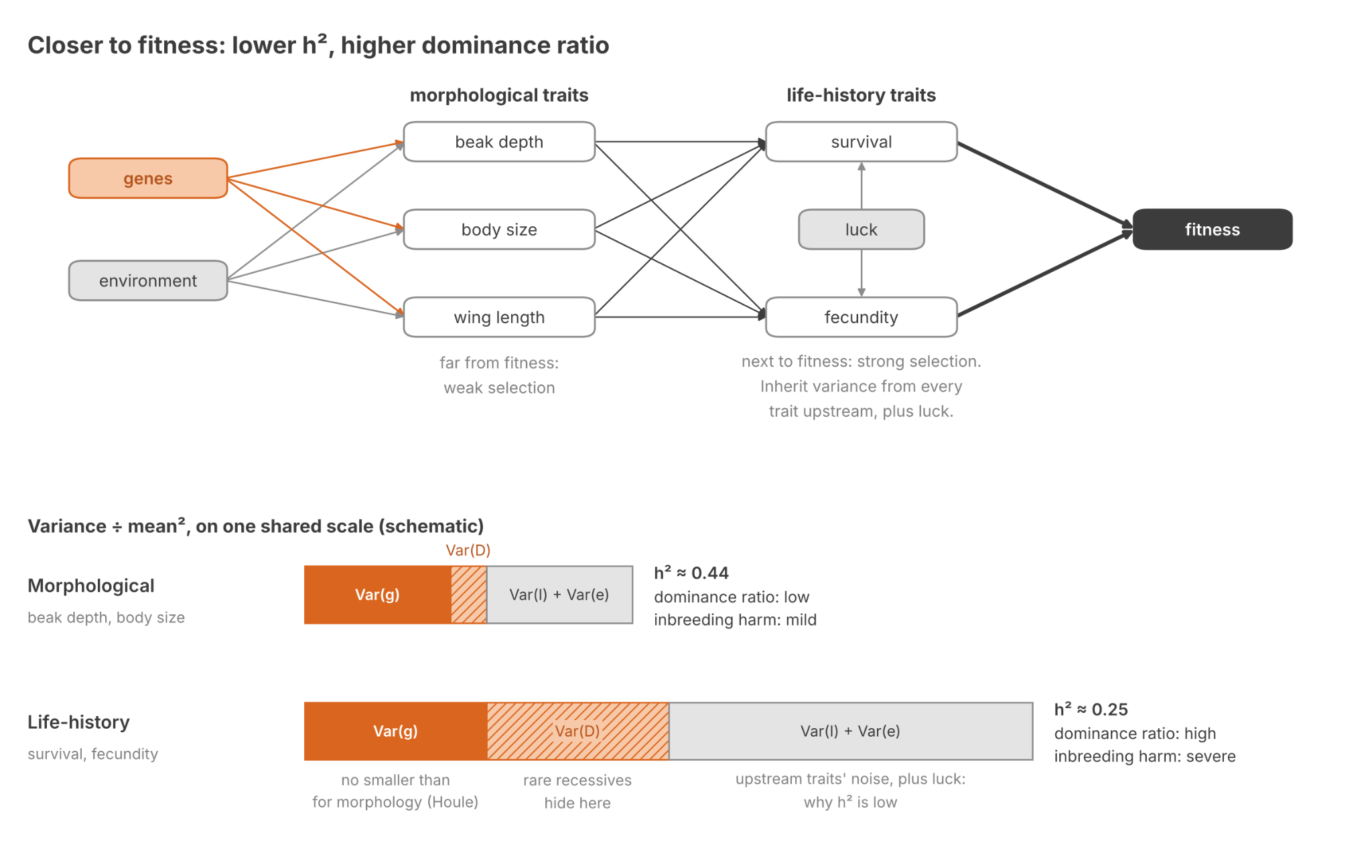
The more fitness-relevant the trait, the higher its dominance ratio tends to be. Life-history (LH) traits such as survival, fecundity and development time are very correlated with fitness. They mediate much of the fitness impact of morphological traits. And indeed, in wild species LH traits have higher dominance ratios (Crnokrak & Roff 1995). In sand crickets, inbreeding harms LH traits far more than it harms body size (Roff 1998). LH traits also have lower heritabilities (Mousseau & Roff 1987), mostly because Var(u) is greater (Houle 1992).

Does selection eventually stall? Mutation resupplies Var(g). But most mutations are harmful, so it also lowers fitness. In the replicator–mutator equation, the two settle into a balance where mean fitness stops rising. Do real populations reach that balance?

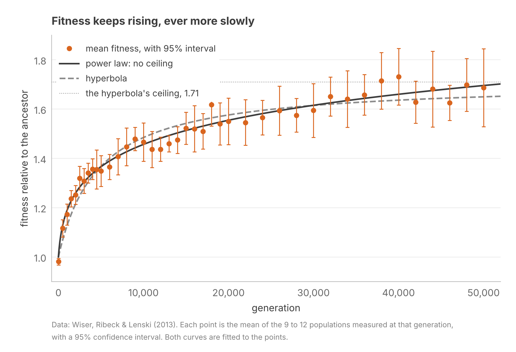
Lenski’s long-term evolution experiment (LTEE) addresses this question. Twelve populations of E. coli have grown in the same glucose-limited medium since 1988. Their fitness rose for 50,000 generations. The data fit a model with no ceiling better than one with a ceiling (Wiser et al 2013). The balance has not yet been reached.

The balance arrives when almost every new mutation is harmful. But a bacterial genome offers a very large search space. The topography of fitness landscapes is such that each selective sweep adds less fitness than the last, but they keep coming (Khan et al 2011).

Lenski’s medium never changes. But in the wild, the world changes too. The theorem does not guarantee an increase in mean fitness. Price (1972) and Frank & Slatkin (1992) showed that Fisher meant only the part of the change that selection causes. Fitness splits into g and u, so its change does too:

R(w) = R(g) + R(u)

For fitness, the assumption that R(u) = 0 breaks down. Offspring inherit their parents’ breeding value for fitness, but not their parents’ world. The climate may change. Rival species may evolve. And fitness can vary with intrapopulation changes, such as density or changes in variant frequencies. Fisher called all of these cases of nonzero R(u) the deterioration of the environment. A population can gain fitness through selection every generation while its mean fitness stays flat.

The Moment Hierarchy

We have finished our survey of models derived from Price. They come in three categories.

Identity models predict nothing. They model a change that has already happened.
One-step models require data on the present population plus rules for fitness and transmission. Their assumptions permit prediction across one generation.
Closed model predictions can be used as new data, which allow for repeat predictions. They allow forecasting change across time.

Why do some of our models reach the third level, while the rest stop at the second? The answer lies in which summaries of the population each model tracks, and whether those summaries predict their own future.

The mean is the first moment of the trait’s distribution: the average of z itself. The kth moment, for k above 1, averages the kth power of each individual’s deviation from the mean:

$\displaystyle \operatorname{E}((z-\bar{z})^k)$

The second moment is the variance. Squaring makes every deviation positive, so it measures spread. The third moment measures skew.

The Price equation updates the first moment, in our case the change in mean beak depth. But two finch populations with the same mean can have dramatically different means after one generation. Consider a population of finches with three variants, each with a distinct beak depth:

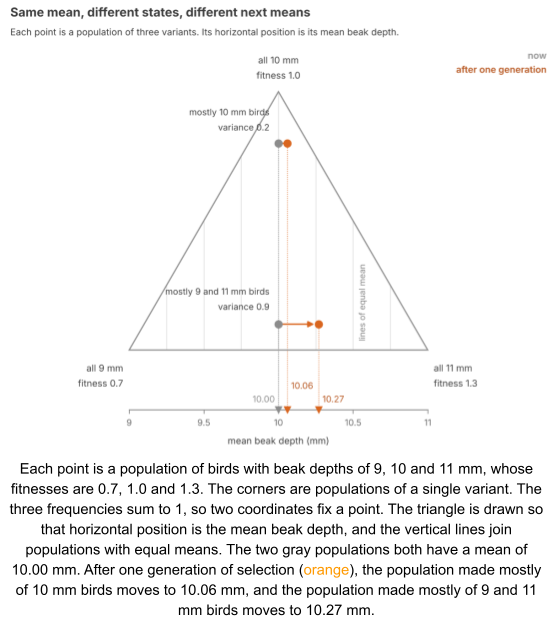
Lewontin (1974) called a set of variables dynamically sufficient when it predicts its own future. With three variants, the mean is not dynamically sufficient. Knowing the mean is not enough to predict how it will change.

To see why, let’s regress w on z. The covariance in S is the slope β of this regression multiplied by the variance:

$S = \frac{\operatorname{Cov}(w,z)}{\bar{w}} = \frac{\beta\,\operatorname{Var}(z)}{\bar{w}}$

So the change in mean depends on variance. And the change in variance under selection depends on skew. Write $Var*(z)$ for the variance after selection. If fitness is a straight line in the trait:

$\displaystyle \operatorname{Var}^{*}(z)-\operatorname{Var}(z) = \frac{\beta \operatorname{E}((z-\bar{z})^3)}{\bar{w}}-S^2$

So two populations with the same first and second moments can still change differently, if their third moments differ.

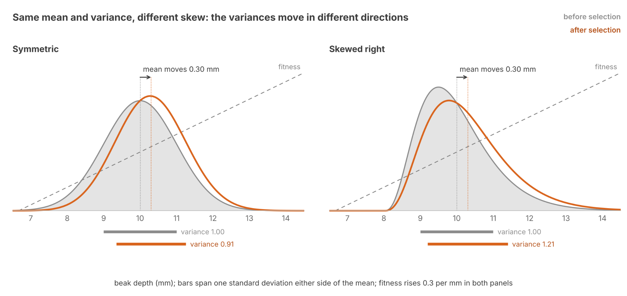
The pattern continues up the chain. The change in each moment depends on the next higher moment. This chain of dependencies is the moment hierarchy. In general, no finite set of moments predicts its own future.

There are two ways to cut the chain and accomplish moment closure, one for discrete traits and one for continuous traits.

Discrete closure is exact. Recall the three-variant triangle above. Switching to two variants, the triangle shrinks to a line segment. If the two variants have beak depths $z₁$ and $z₂$ , and the first has frequency x, the mean is:

$\bar{z} = x\,z_1 + (1-x)\,z_2$

Solve for x. Since z₁ and z₂ are fixed, the frequency follows from the mean alone (as long as the denominator is nonzero).

$x = \frac{\bar{z}-z_2}{z_1-z_2}$

So the variance is also a function of the mean alone:

$\operatorname{Var}(z) = x(1-x)(z_1-z_2)^2 = (\bar{z}-z_2)(z_1-\bar{z})$

We saw that S needs the variance. But the variance only needs the mean. The chain closed after the first moment.

But as the triangle showed, with three variants the mean is not dynamically sufficient. In such cases, we can achieve closure by instead using indicator variables for each variant. Their means are the variant frequencies, and together the frequencies fix the population. Writing the Price equation once per indicator gives the replicator–mutator equation.

We defined a variant as having members with the same fitness and the same kinds of offspring. So for each variant, W and Q are fixed tables, or depend only on the frequencies, and w̄ is determined from variant frequencies. The equation updates frequencies, and can be iterated to forecast into future generations. Population genetics models are closed models.

Continuous closure is approximate. Without a finite list of variants, the chain must be cut by assumptions. The usual ones are that the trait stays normal and its variance stays steady. A normal distribution is fixed by its mean and variance. If the assumptions hold, dynamic sufficiency is obtained.

$R = h²S$ gives the response for one generation. To predict the next, the breeder’s equation assumes that h² and the variance of the trait stay the same. Selection changes both. Holding h² and the variance fixed cuts the chain, so the mean can predict its own future.

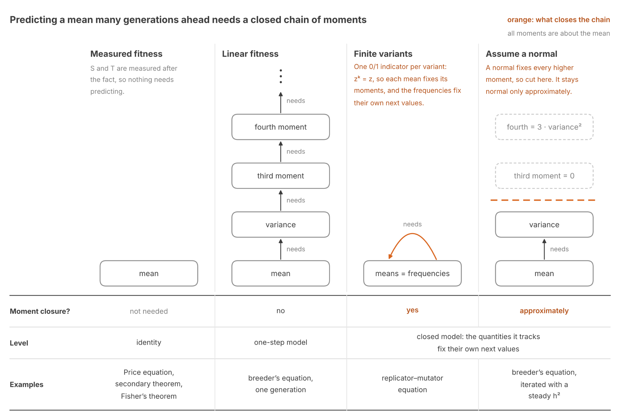
Continuous closure requires assumptions. What reason do we have to believe they are valid? Fisher (1918) answered with the infinitesimal model: a trait is the sum of the small effects of a large number of genes. Discrete closure is impractical here. A gene’s fitness depends on the genes it is paired with, so it would need one indicator per combination of genes, and there are astronomically many. However, by the central limit theorem, such a sum is close to normal. And because each gene’s effect is small, selection barely changes any gene’s frequency, so after an initial drop the variance holds steady. So the infinitesimal model generates conditions which make continuous closure’s assumptions approximately true.

The infinitesimal model is supported by modern genomic data. Genes of large effect do exist. In medium ground finches, one gene, HMGA2, has a large effect on beak size, and selection on it was strong during a later drought (Lamichhaney et al 2016). But genome-wide association studies (GWAS), which scan the whole genome for variants associated with a trait, have revealed that most complex traits are highly polygenic. For example, more than ten thousand variants together explain about 40% of the variance in height among people of European ancestry (Yengo et al 2022).

Applications

Our discussion so far has been fairly theoretical. Let’s close with some practical use cases.

First, let’s consider fisheries-induced evolution. Historically, fisheries usually bring the largest fish to market. This has the unfortunate side effect of leaving smaller fish to breed: selection for small body size. Since body size is heritable, the breeder’s equation predicts smaller fish in the next generation. Conover & Munch (2002) confirmed this in captive Atlantic silversides. The breeder’s equation also points to the remedy. Managers cannot change h², but they choose S. Catching fish at random brings S to zero, and purposefully releasing the largest fish makes it positive.

Second, animal breeders historically selected on the basis of traits like milk yield. But genomic selection estimates an animal’s g from its DNA at birth (Meuwissen et al 2001). By using information from the genotype instead of the phenotype, breeders can choose parents years earlier. Generations got shorter, and yearly gains rose by 50–100% for yield traits. Gains were especially pronounced for low heritability traits, where an animal’s own phenotype reveals little about its g (García-Ruiz et al 2016).

These theorems of evolution apply in situations not involving nucleic acids. Price (1995) called for a universal selection theory that would treat chemical, cultural and genetic selection alike, the way communication theory treats every kind of signal.

Does an economy grow because firms improve their own productivity, or because they outcompete other firms? Economists answer with the Price equation. Treat each firm’s productivity as the trait z, and its share of the industry’s output as its frequency x. Then S is reallocation: output shifting from unproductive to productive firms. T is self-improvement. Since a new firm has no parent, firm entry needs a term of its own. Firm turnover (entry and exit) shows up in both S and the entry term.

The answer depends on the industry. In 1980s US manufacturing, about 80% of productivity growth was T (Foster et al 2001). In 1990s US retail, virtually all labor productivity growth came from turnover: new stores replacing less productive ones (Foster et al 2006).

In industries where growth depends on turnover, keeping weak firms alive is costly. In 1990s Japan, banks kept lending to failing “zombie” firms. Industries full of zombies had lower productivity, and fewer healthy firms entered (Caballero et al 2008). In Price’s terms, without the loans the fitness of zombie firms would have been zero.

The contrast with biology is in transmission T. For beak depth, T is regression to the mean. Chicks inherit only the fraction h² of their parents’ advantage. So S does the work, and T gives part of it back. But for firms, T can be positive and drive most of an industry’s growth. T averages each firm’s change in productivity from its earlier self. While mutation is blind, firms change on purpose. Change that is aimed at improvement and then passed on is called guided variation (Boyd & Richerson 1985). Guided variation can make T positive without any selection: firms improve even if their shares never change.

Wrapping Up

We learned the following today.

The Price equation splits a response R of a variable into the selection differential S and transmission T. It holds for any trait and any rule of inheritance. It is an identity. But with rules for fitness and transmission, it can become a predictive model.
With an indicator for each variant, the Price equation becomes the replicator–mutator equation.
Tracking the breeding value g instead of the phenotype z removes T, leaving only S. This is Robertson’s secondary theorem.
The breeder’s equation says that only the fraction h² of S reaches the offspring.
Applied to fitness, the Price equation becomes Fisher’s fundamental theorem. Variance in heritable fitness is the fuel of selection.
Predicting many generations needs a closed model. Discrete traits can afford exact moment closure. Continuous traits can be closed approximately, through the infinitesimal model.

Until next time.

References

Arnold & Wade (1984). On the measurement of natural and sexual selection: theory.
Boag (1983). The heritability of external morphology in Darwin’s ground finches (Geospiza) on Isla Daphne Major, Galápagos.
Boyd & Richerson (1985). Culture and the evolutionary process.
Caballero et al (2008). Zombie lending and depressed restructuring in Japan.
Conover & Munch (2002). Sustaining fisheries yields over evolutionary time scales.
Crnokrak & Roff (1995). Dominance variance: associations with selection and fitness.
Fisher (1918). The correlation between relatives on the supposition of Mendelian inheritance.
Fisher (1930). The Genetical Theory of Natural Selection.
Foster et al (2001). Aggregate productivity growth: lessons from microeconomic evidence.
Foster et al (2006). Market selection, reallocation, and restructuring in the U.S. retail trade sector in the 1990s.
Frank & Slatkin (1992). Fisher’s fundamental theorem of natural selection.
Galton (1886). Regression towards mediocrity in hereditary stature.
García-Ruiz et al (2016). Changes in genetic selection differentials and generation intervals in US Holstein dairy cattle as a result of genomic selection.
Grant (1986). Ecology and Evolution of Darwin’s Finches.
Grant & Grant (1995). Predicting microevolutionary responses to directional selection on heritable variation.
Grant & Grant (1996). Cultural inheritance of song and its role in the evolution of Darwin’s finches.
Houle (1992). Comparing evolvability and variability of quantitative traits.
Khan et al (2011). Negative epistasis between beneficial mutations in an evolving bacterial population.
Kingsolver et al (2001). The strength of phenotypic selection in natural populations.
Kruuk et al (2002). Antler size in red deer: heritability and selection but no evolution.
Lamichhaney et al (2016). A beak size locus in Darwin’s finches facilitated character displacement during a drought.
Lewontin (1974). The Genetic Basis of Evolutionary Change.
Merilä et al (2001). Explaining stasis: microevolutionary studies in natural populations.
Meuwissen et al (2001). Prediction of total genetic value using genome-wide dense marker maps.
Mousseau & Roff (1987). Natural selection and the heritability of fitness components.
Price (1970). Selection and covariance.
Price (1972). Fisher’s “fundamental theorem” made clear.
Price (1995). The nature of selection.
Queller (2017). Fundamental theorems of evolution.
Robertson (1966). A mathematical model of the culling process in dairy cattle.
Roff (1998). Effects of inbreeding on morphological and life history traits of the sand cricket, Gryllus firmus.
Schulman et al (2012). Robust self-replication of combinatorial information via crystal growth and scission.
Wiser et al (2013). Long-term dynamics of adaptation in asexual populations.
Yengo et al (2022). A saturated map of common genetic variants associated with human height.

Appendix A: Deriving the Price Equation

This appendix derives the two steps of The Fundamental Theorem of Evolution. It uses the rules for counting chicks by their parent’s class, and the parents’ mean counted once per chick:

$\displaystyle x_i^{\prime} = \frac{x_i w_i}{\bar{w}}, \quad z_i^{\prime} = z_i+\varDelta z_i, \quad \bar{z}^{*} = \sum_i x_i^{\prime} z_i$

Start with the first step. Substitute the rule for xᵢ′ into z̄*:

$\bar{z}^{*} = \sum_i \frac{x_i\,w_i}{\bar{w}}\,z_i = \frac{\operatorname{E}(wz)}{\bar{w}}$

The covariance of fitness and trait is the average product of their deviations (see The Reliability Ratio). Expanding that product gives a shorter form:

$\operatorname{Cov}(w,z) = \operatorname{E}(wz)-\bar{w}\,\bar{z}$

Subtract z̄ from z̄*, writing both over w̄, and use the shorter form:

$\bar{z}^{*}-\bar{z} = \frac{\operatorname{E}(wz)-\bar{w}\,\bar{z}}{\bar{w}} = \frac{\operatorname{Cov}(w,z)}{\bar{w}}$

Now the second step. Substitute the rule for zᵢ′. The zᵢ parts cancel:

$\displaystyle \bar{z}^{\prime}-\bar{z}^{*} = \sum_i x_i^{\prime} (z_i+\varDelta z_i)-\sum_i x_i^{\prime} z_i = \sum_i x_i^{\prime} \varDelta z_i$

Substitute the rule for xᵢ′:

$\displaystyle \sum_i x_i^{\prime} \varDelta z_i = \frac{\sum_i x_i w_i \varDelta z_i}{\bar{w}} = \frac{\operatorname{E}(w \varDelta z)}{\bar{w}}$

Add the two steps:

$\displaystyle \varDelta\bar{z} = \frac{\operatorname{Cov}(w,z)}{\bar{w}} + \frac{\operatorname{E}(w \varDelta z)}{\bar{w}}$

Appendix B: Deriving the Replicator–Mutator Equation

This appendix derives the left branch of the tree in full. Let z be the indicator for variant i: 1 for variant i, and 0 for every other variant. Its mean is the frequency of variant i:

$\bar{z} = x_i$

The same holds among offspring, so the left side of the Price equation becomes:

$\displaystyle \varDelta\bar{z} = \bar{z}^{\prime}-\bar{z} = x_i^{\prime}-x_i = \varDelta x_i$

Start with T. An offspring of a variant-k parent lands in variant i with probability $\textstyle Q_{ik}$ . That probability is the mean z of its offspring, so the change in z for a variant-k parent is:

$\displaystyle \varDelta z_k = Q_{ik}-z_k$

Substitute the change in z into T. Only variant i has z = 1:

$\displaystyle \frac{\operatorname{E}(w \varDelta z)}{\bar{w}} = \frac{\sum_k x_k w_k (Q_{ik}-z_k)}{\bar{w}} = \frac{\sum_k Q_{ik} w_k x_k}{\bar{w}}-\frac{x_i w_i}{\bar{w}}$

Split off the offspring of variant i that stay in variant i:

$\frac{\sum_k Q_{ik}\,w_k\,x_k}{\bar{w}}-\frac{x_i\,w_i}{\bar{w}} = \frac{\sum_{k\neq i} Q_{ik}\,w_k\,x_k}{\bar{w}}-\frac{(1-Q_{ii})\,w_i\,x_i}{\bar{w}}$

The first part counts offspring that mutate into variant i, and the second counts offspring of i that mutate out:

$\displaystyle \frac{\operatorname{E}(w \varDelta z)}{\bar{w}} = \text{mutation in}-\text{mutation out} = \frac{\sum_{k\neq i} Q_{ik} w_k x_k}{\bar{w}}-\frac{(1-Q_{ii}) w_i x_i}{\bar{w}}$

Next, S. Recall the shorter form of the covariance from Appendix A:

$\operatorname{Cov}(w,z) = \operatorname{E}(wz)-\bar{w}\,\bar{z}$

Only variant i has z = 1, so only its fitness enters the average of wz:

$\operatorname{E}(wz) = x_i\,w_i$

Substitute E(wz) and z̄ into S:

$\frac{\operatorname{Cov}(w,z)}{\bar{w}} = \frac{x_i\,w_i-\bar{w}\,x_i}{\bar{w}} = x_i\,\frac{w_i-\bar{w}}{\bar{w}}$

Finally, add S and T. By the Price equation, the change in frequency is their sum:

$\displaystyle \varDelta x_i = \frac{\operatorname{Cov}(w,z)}{\bar{w}}+\frac{\operatorname{E}(w \varDelta z)}{\bar{w}}$

Substitute S and T and add xᵢ:

$x_i^{\prime} = x_i+x_i\,\frac{w_i-\bar{w}}{\bar{w}}+\frac{\sum_k Q_{ik}\,w_k\,x_k}{\bar{w}}-\frac{x_i\,w_i}{\bar{w}}$

Every term except the flow through Q cancels:

$x_i^{\prime} = \frac{\sum_k Q_{ik}\,w_k\,x_k}{\bar{w}}$

In matrix form, with W the diagonal matrix of fitnesses, this is the replicator–mutator equation in frequencies:

$x^{\prime} = \frac{QWx}{\bar{w}}$

If each variant breeds true, Q is the identity matrix and T vanishes. The sum for xᵢ′ then keeps only its k = i term, which is the replicator equation:

$x_i^{\prime} = x_i\,(w_i/\bar{w})$

With two variants, the Price equation can be iterated, and this derivation recovers the mutation–selection balance of Intro to Replicator Dynamics without its approximation. Take the model from that post. The original variant has fitness 1, and a harmful mutant has fitness cost s. Each offspring of an original parent is a mutant with probability μ, and there are no mutations back to the original. Let variant i be the mutant, and write x for its frequency. Mean fitness is:

$\bar{w} = (1-x)\cdot 1+x\,(1-s) = 1-sx$

Substitute the mutant’s fitness and mean fitness into S:

$\frac{\operatorname{Cov}(w,z)}{\bar{w}} = \frac{x\,[(1-s)-(1-sx)]}{1-sx} = -\frac{s\,x\,(1-x)}{1-sx}$

In T, mutation in is the offspring of original parents that mutate. Mutation out is zero, because no offspring of a mutant mutates back:

$\displaystyle \frac{\operatorname{E}(w \varDelta z)}{\bar{w}} = \text{mutation in}-\text{mutation out} = \frac{\mu (1-x)}{1-sx}-0$

By the Price equation, Δx is the sum of S and T:

$\displaystyle \varDelta x = \frac{\mu (1-x)}{1-sx}-\frac{s x (1-x)}{1-sx}$

Collect the common factor:

$\displaystyle \varDelta x = \frac{(1-x)(\mu-s x)}{1-s x}$

The right side depends on x alone, and x is the whole state, because the original makes up the rest of the population. So the output of each step can be fed back in as the next step’s input.

Intro to Replicator Dynamics wrote this change as inflow minus outflow, with mutation as the inflow and selection as the outflow. In terms of S and T, these are:

$\displaystyle \text{inflow} = \frac{\operatorname{E}(w \varDelta z)}{\bar{w}} = \frac{\mu (1-x)}{1-sx}$

$\text{outflow} = -\frac{\operatorname{Cov}(w,z)}{\bar{w}} = \frac{s\,x\,(1-x)}{1-sx}$

This outflow is selection, not mutation out of the mutant, which is zero here. Both flows carry the same factor, which is close to 1 while the mutant is rare. Setting it to 1 gives that post’s approximation:

$\displaystyle \varDelta x = \text{inflow}-\text{outflow} \approx \mu-sx$

The common factor is positive whenever some originals remain, so it changes how fast the frequency moves, but not where it stops. So that post’s equilibrium needs no approximation:

$x^{*} = \frac{\mu}{s}$

The factor’s 1 − x adds one more fixed point:

$x^{*} = 1$

A population of only mutants stays that way, since no mutant mutates back. When μ < s, any population that still has some originals moves away from it, toward μ/s. When μ ≥ s, the mutant takes over.

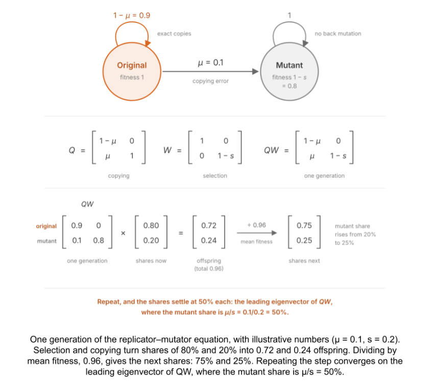
The replicator–mutator figure in that post took μ = 0.1 and s = 0.2, and moved the mutant from 20% to 25% of the population in one generation. At x = 0.2, the factored line gives that step:

$\displaystyle \varDelta x = \frac{(1-0.2)(0.1-0.2\times 0.2)}{1-0.2\times 0.2} = \frac{0.8\times 0.06}{0.96} = 0.05$

The approximation would give 0.06. Iterated, the frequency settles at μ/s, which is 50%, as in that figure.

Appendix C: Deriving the Breeder’s Equation

This appendix derives the breeder’s equation from Robertson’s secondary theorem. The first two assumptions of The Breeder’s Equation, u independent of g and both normally distributed, give Kelley’s rule:

$\operatorname{E}(g \mid z) = \bar{g} + h^2\,(z-\bar{z})$

The third assumption is that fitness depends on g only through z:

$\operatorname{E}(w \mid z, g) = \operatorname{E}(w \mid z)$

Recall that w = f(z) + ε, with f(z) the expected fitness at beak depth z. By the third assumption, ε averages to zero at every z and g, so apart from drift it has no covariance with g:

$\displaystyle \operatorname{Cov}(w,g) = \operatorname{Cov}(f(z),g)$

f(z) depends on z alone, so only the average g at each beak depth matters:

$\displaystyle \operatorname{Cov}(f(z),g) = \operatorname{Cov}(f(z),\operatorname{E}(g \mid z))$

Substitute Kelley’s rule. The constant terms drop out of the covariance:

$\displaystyle \operatorname{Cov}(f(z),\operatorname{E}(g \mid z)) = h^2 \operatorname{Cov}(f(z),z)$

ε has no covariance with beak depth, apart from drift, so f(z) can go back to w:

$\displaystyle h^2 \operatorname{Cov}(f(z),z) = h^2 \operatorname{Cov}(w,z)$

Chained together, these lines convert Robertson’s covariance into one we can measure:

$\operatorname{Cov}(w,g) = h^2\,\operatorname{Cov}(w,z)$

Divide both sides by w̄:

$S(g) = h^2 S$

Robertson’s theorem makes S(g) the response of g:

$R(g) = h^2 S$

Recall that z = g + u. This splits the response to selection:

$R = R(g) + R(u) = h^2 S + R(u)$

The second assumption of The Theorem of Phenotype Selection removes the last term:

$R = h^2 S$

Intro to Replicator Dynamics

October 18, 2026October 20, 2026kevinbinz 2 Comments

Part Of: Biology sequence
Related To: Population Genetics, Natural Selection, Fitness Seascapes
Content Summary: 4400 words, 22 min read

Introduction

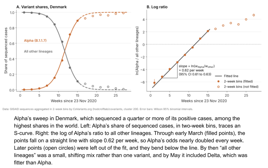
In January 2021, the Alpha variant of SARS-CoV-2 made up less than half a percent of US cases. The CDC projected that it would become the dominant variant by March (Galloway et al. 2021). By early April, it was the most common lineage in the US. The forecast didn’t need to model immune systems or social networks in detail. Its central driver was simply how much faster Alpha spread than other variants.

This suffices because variants are self-replicators. Advantages in exponential growth compound. The replicator equation is a simple way to model such processes.

Evolution is usually told as a story about DNA, but the replicator equation never mentions nucleic acid. The natural world is rife with many other replicators, and the replicator equation applies to all of them.

This post develops the replicator equation in its simplest form, and then relaxes its assumptions. We allow fitness to change, mutation to add new variants, and finally finite populations to introduce sampling. Each change can enrich the forecast.

Let’s dive in!

The Replicator Equation

A self-replicator makes more of itself, and each copy makes copies of its own. This entails positive feedback: the more copies exist, the faster new ones appear. When every copy replicates at a fixed pace, the population undergoes exponential growth, doubling at regular intervals. We define fitness w as the number of copies that each replicator leaves per generation.

Consider two strains of E. coli in a flask. Let’s suppose strain A has a doubling time of 30 minutes, and strain B has 20 minutes. All cells replicate at the rate prescribed by their strain identity. The strain of the parents is transmitted to their offspring. Each strain therefore breeds true.

A class of individuals that shares a fitness and breeds true is a variant. Not every class qualifies. “Large cells” does not breed true, because a large cell divides into two small ones. “All cells in the flask” breeds true, but its members do not share the same fitness. In sexually reproducing organisms, a genotype does not breed true, because sex reshuffles the genome.

Heritable state is whatever makes an offspring resemble their parent. In clonal bacteria, the heritable state is the genome. In sexual species, it is the allele. Heritable state can also be the composition of a chemical network, or a handwritten note.

Each variant i multiplies by its own fitness wᵢ every generation. Both strain populations grow. But strain B’s fraction of the flask grows toward 100%. More generally, the frequency $xᵢ = nᵢ/N$ obeys the replicator equation:

$x_i’ = x_i\frac{w_i}{\bar{w}}$

Here $w̄ = Σⱼxⱼwⱼ$ is the mean fitness and $wᵢ/w̄$ is the relative fitness of the variant. A variant grows when it is fitter than average and shrinks when it is less fit.

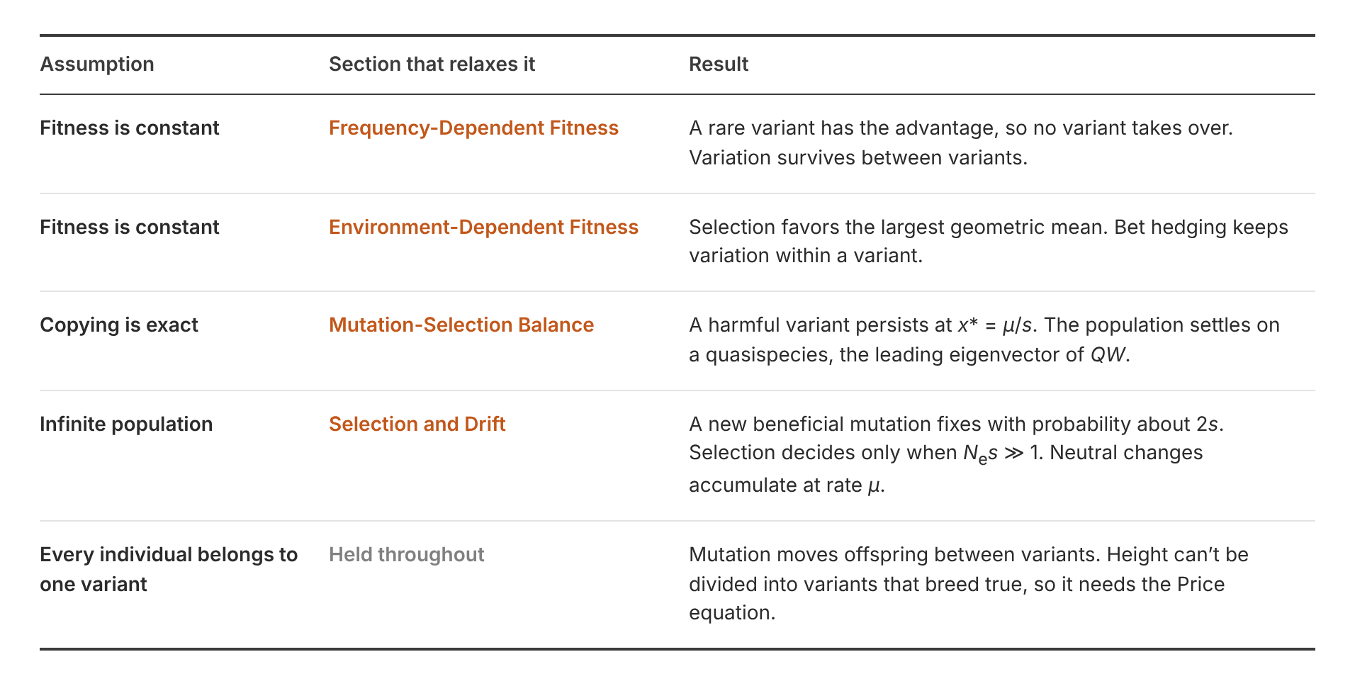
The replicator equation makes four assumptions:

Fitness is constant.
Copying is exact. Every offspring inherits the variant of its parent.
An infinite population. This entails no genetic drift.
Every individual belongs to exactly one variant.

The replicator equation describes real selective sweeps, with a fitter variant replacing its rivals. Each generation multiplies the odds of variant 1 against variant 2 by $w₁/w₂$ :

$\ln\frac{x_1′}{x_2′} = \ln\frac{x_1}{x_2} + \ln\frac{w_1}{w_2}$ $\displaystyle \ln\frac{x_1′}{x_2′} = \ln\frac{x_1}{x_2} + \ln\frac{w_1}{w_2}$

Mean fitness cancels, so only fitness ratios matter. On a plot of frequency, a variant with higher relative fitness traces an S-curve. On a plot of log ratio, it traces a straight line.

Under these assumptions, the fittest variant takes over: the variation disappears. Selection consumes the variation it runs on.

Density-Dependent Fitness

The replicator equation assumes that fitness is constant. What happens when a replicator’s fitness depends on how many copies there are?

Szathmáry (1991) wrote the growth of a variant with n copies in terms of its total rate, the number of new copies per unit time, summed over all copies:

$\text{total rate} = \frac{dn}{dt} = k\,n^{p}$

Here k is a rate constant, and the exponent p sets how growth scales with n.

Fitness is the per-capita rate: new copies per copy. Dividing by n gives

$\text{per-capita rate} = \frac{1}{n}\frac{dn}{dt} = k\,n^{p-1}$

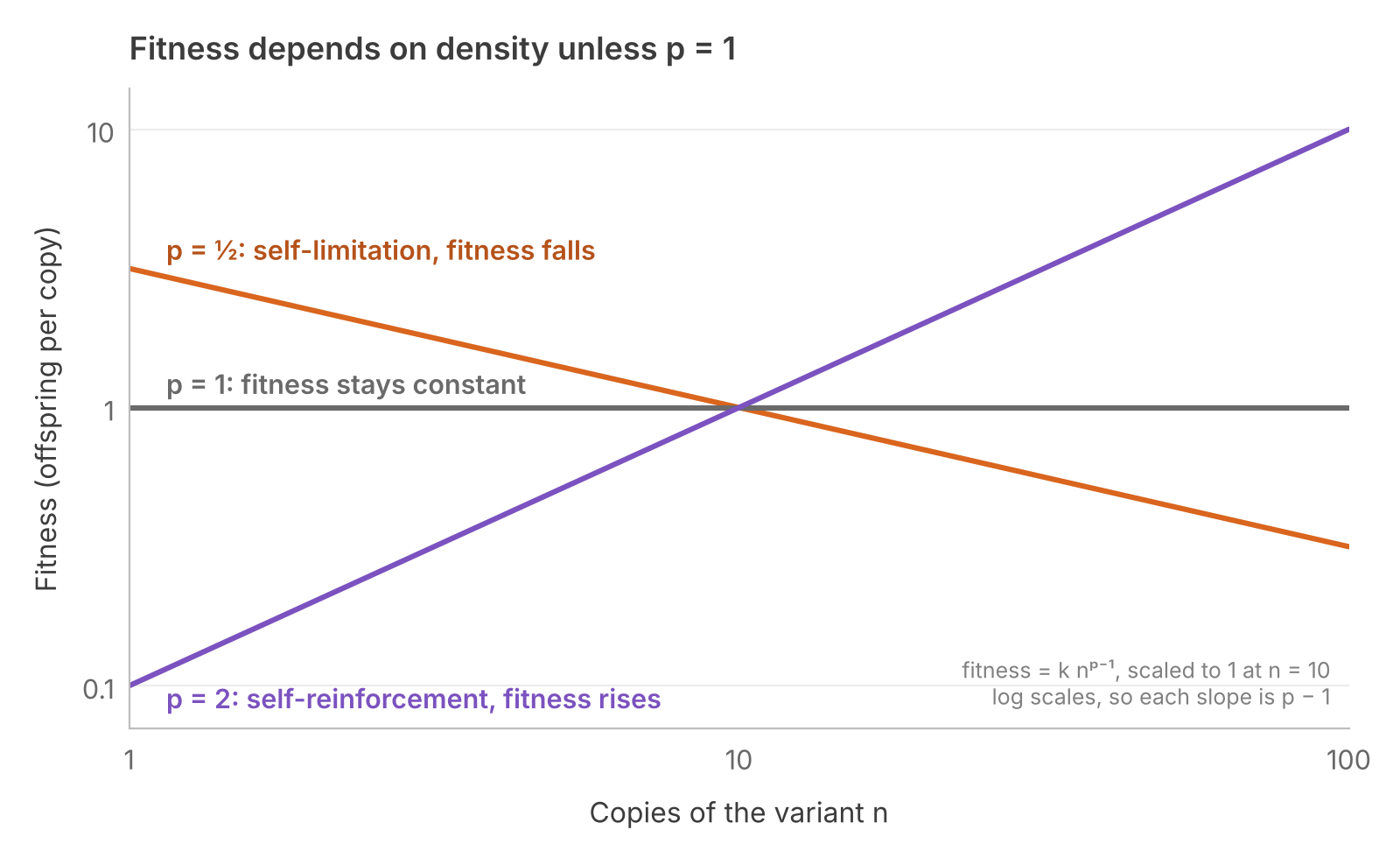
When p = 1, fitness is k at every n. The total rate still rises with n, but only because more copies divide at the same pace. This is density-independent growth, the case the replicator equation assumes. For any other p, fitness depends on n, and growth is density-dependent.

This gives three regimes, and each has its own mechanism.

p < 1: self-limitation. Copies of the variant hold one another back. In a colony, only cells at the rim have room to divide. On a flat dish, the rim grows with the radius while n grows with the area, so the rim holds about √n cells, and p = ½.
p = 1: independence. Copies neither crowd nor help one another, as for bacteria in a flask with nutrients in excess.
p > 1: self-reinforcement. Copies help one another replicate. A replicator whose product catalyses its own copying needs two of its copies to meet, so p is about 2. Ecologists call the same pattern an Allee effect: some animals breed better in larger groups.

Solved over time, the growth law gives each regime its name. Growth is called subexponential when p < 1, and exponential when p = 1. It is called superexponential when p > 1, and it then runs to infinity in finite time. Real growth stops before then, when something else runs out.

Now let two variants compete, each with its own rate constant and the same p. The log-ratio equation still applies, in its continuous-time form, with density-dependent fitness substituted:

$w_i = k_i\,n_i^{\,p-1}$

$\frac{d}{dt}\ln\frac{n_1}{n_2} = k_1\,n_1^{\,p-1}-k_2\,n_2^{\,p-1}$

Szathmáry (1991) named the three outcomes.

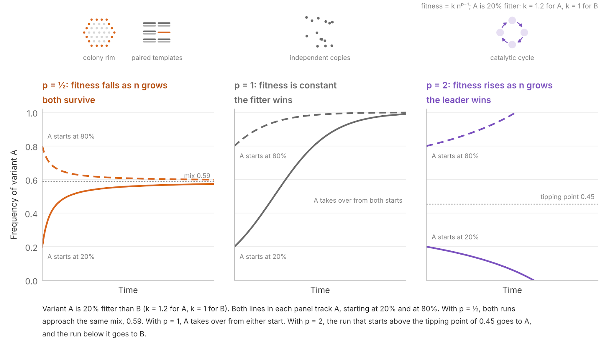
p < 1: survival of everybody. A variant’s fitness falls as it becomes common, so the ratio moves to where the two fitnesses match. For p = ½, that is n₁/n₂ = (k₁/k₂)². Both variants survive, from any start (Szathmáry & Gladkih 1989).
p = 1: survival of the fittest. The right side is the constant k₁ − k₂, so the fitter variant takes over, as in the replicator equation.
p > 1: survival of the first. A variant’s fitness rises as it becomes common, so the variant ahead pulls further ahead. Variant 1 gains only while n₁/n₂ exceeds (k₂/k₁)^(1/(p − 1)). A less fit variant that starts far enough ahead stays ahead. This is lock-in.

This density dependence is specific to each variant. Dilution in a chemostat removes copies of every variant at the same per-capita rate, so it cancels from the log-ratio equation at every instant.

Frequency-Dependent Fitness

Fitness can also depend on the composition of the population. In the hawk–dove game (Maynard Smith & Price 1973; Maynard Smith 1982), two animals contest a prize worth B. Hawks fight, and the loser pays C. Doves share with doves and retreat from hawks. Each entry is the row player’s expected payoff against the column player:

$\begin{array}{c|cc} & \text{Hawk} & \text{Dove} \\ \hline \text{Hawk} & \frac{B-C}{2} & B \\ \text{Dove} & 0 & \frac{B}{2} \end{array}$

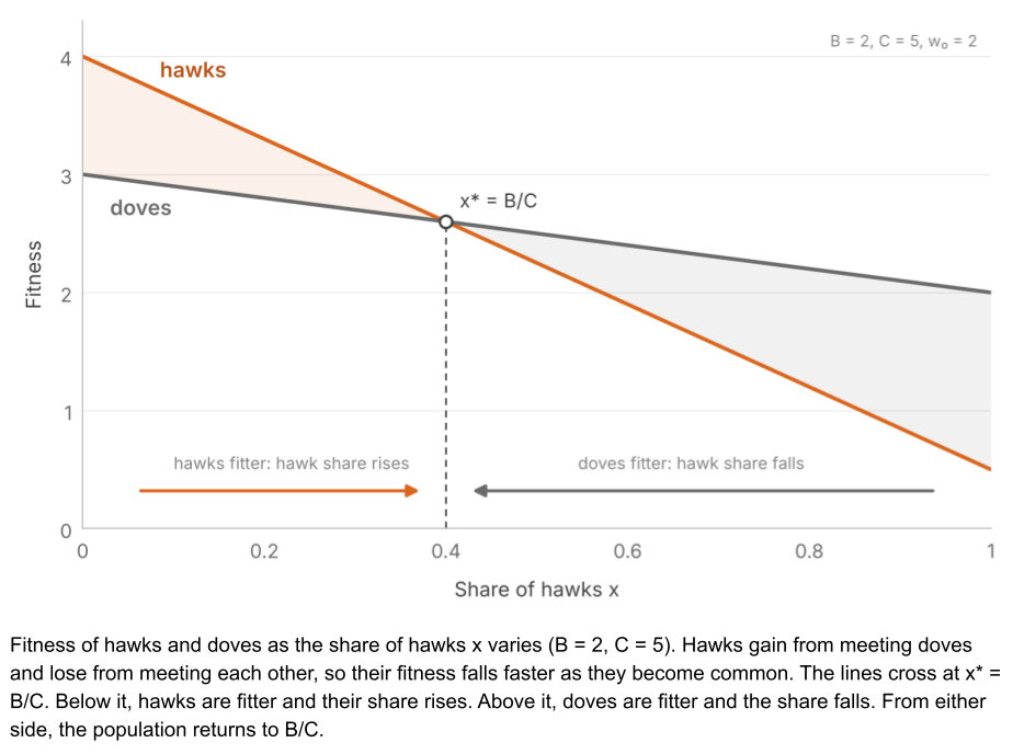
When a fight costs more than the prize ( $C > B$ ), hawks do well among doves and badly among hawks. Let x be the share of hawks, and let each animal meet a random opponent. Each strategy’s fitness is a baseline w₀ plus its average payoff, so the hawks’ advantage

$w_H – w_D = x\frac{B-C}{2} + (1-x)\frac{B}{2} = \frac{B-xC}{2}$

This advantage is positive while hawks are rarer than $B/C$ and negative once they are more common. Each strategy does best when it is rare. The population settles where hawks make up $B/C$ of it. Evolutionary game theory develops such games in more detail.

Ecology has a well-known counterpart. Competitive exclusion (Gause 1934) states that two species limited by one resource cannot coexist. Species escape it when each limits its own growth more than it limits the other’s, so that each species has an advantage when rare (Chesson 2000).

The two models are one system in different coordinates. When fitness depends linearly on frequencies, the continuous-time replicator equation for n variants (Taylor & Jonker 1978) becomes the Lotka–Volterra equations for n − 1 species (Hofbauer 1981).

Environment-Dependent Fitness

Fitness can also depend on the environment, so that wᵢ is a function of time. Then the forecast must average over good years and bad ones, and the right average is not the obvious one.

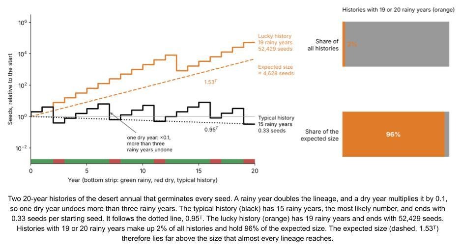
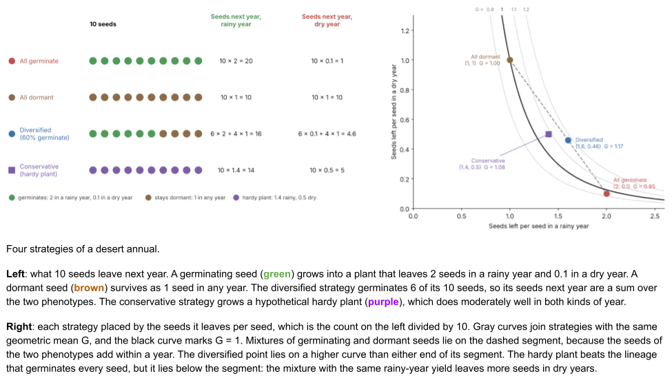
Consider a desert annual plant. Rain falls in 75% of years ( $π = 0.75$ ). In a rainy year, a plant makes two seeds ( $w_{\text{rain}} = 2$ ). In a dry year, the plant leaves 0.1 seeds on average ( $w_{\text{dry}} = 0.1$ ). Let’s assume that the climate is unpredictable. Let one year be one generation.

Let each member of variant i leave $wᵢ(t)$ offspring in year t. After T years, its lineage has grown by the product of these fitnesses. The geometric mean fitness Gᵢ is the constant yearly fitness that produces the same growth:

$G_i = \left(\prod_{t=1}^{T} w_i(t)\right)^{1/T}$

So each lineage grows by $Gᵢᵀ$ , and the variant with the largest G takes over.

Taking the log turns the product into an average, the same form as the arithmetic mean fitness Aᵢ:

$A_i = \frac{1}{T}\sum_{t=1}^{T} w_i(t) \to E[w_i]$

$\displaystyle \ln G_i = \frac{1}{T}\sum_{t=1}^{T} \ln w_i(t) \to E[\ln w_i]$ $\ln G_i = \frac{1}{T}\sum_{t=1}^{T} \ln w_i(t) \to E[\ln w_i]$

As T grows, both averages approach these limits when each year’s environment is drawn independently from a fixed distribution. Because ln G approaches $\textstyle E[\ln w]$ , selection favors the variant with the largest expected log fitness.

For the desert annual that germinates every seed:

$A = \pi w_{\text{rain}} + (1-\pi) w_{\text{dry}} = 0.75 \times 2 + 0.25 \times 0.1 \approx 1.53$

$G = w_{\text{rain}}^{\pi} \times w_{\text{dry}}^{1-\pi} = 2^{0.75} \times 0.1^{0.25} \approx 0.95$

Recall that a plant leaves 2.0 or 0.1 seeds depending on the rain. Scaling by the natural log, a rainy year adds 0.69 and a dry year subtracts 2.30 log fitness. A dry year cancels the effect of more than three rainy years! This result derives from Jensen’s inequality where, for any concave function f,

$E[f(x)] \le f(E[x])$

Since logarithms are concave:

\displaystyle \ln G = E[\ln w] \le \ln E[w] = \ln A

So G < A whenever fitness varies.

The means answer different questions. The arithmetic mean is an ensemble average: lineage size across every possible sequence. The geometric mean is a time average, lineage size across very long experiences of a single variant. Ergodicity holds when ensemble and time averages agree (Peters & Gell-Mann 2016).

Compounding growth lacks ergodicity, so the arithmetic mean misleads. Lewontin & Cohen (1969) showed that a population like our desert annual can grow in expected size, while its extinction is almost certain.

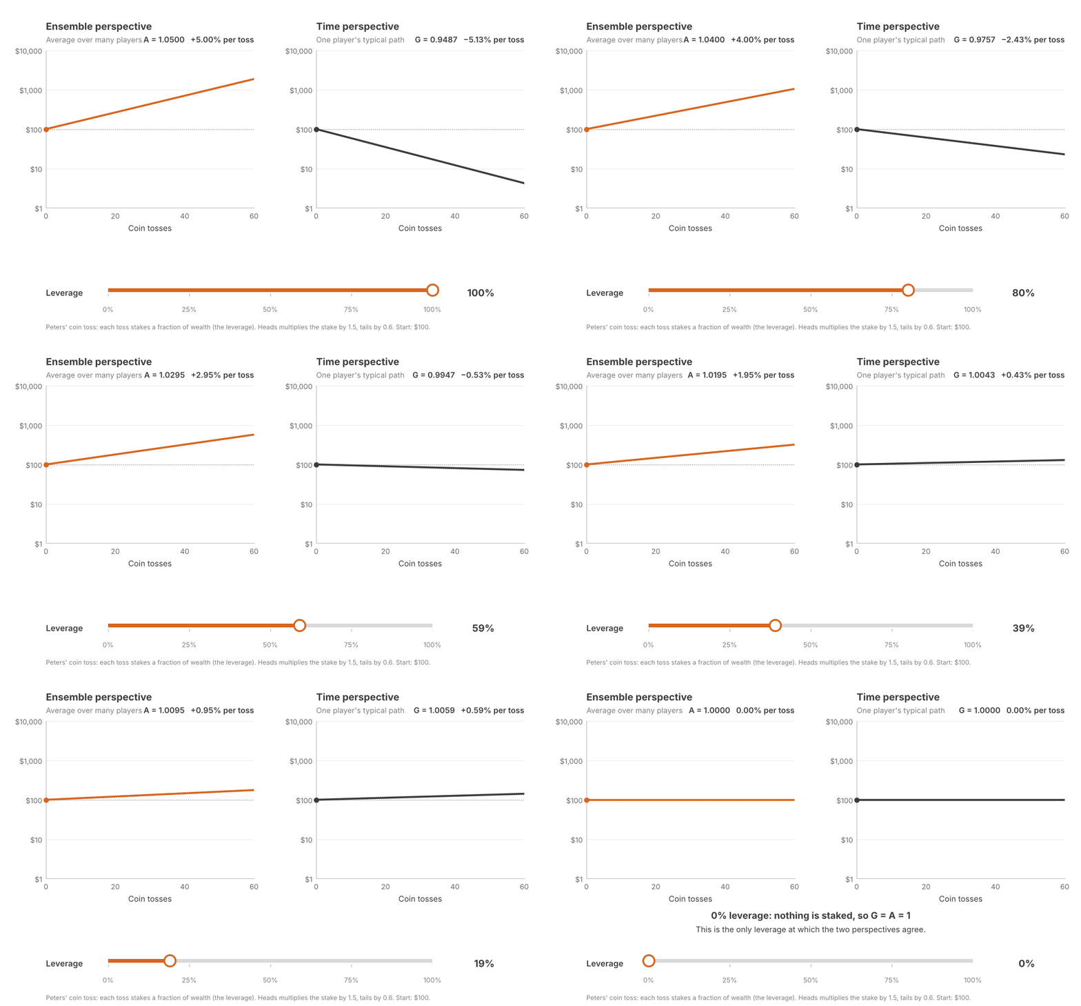
Finance also features exponential growth. In that field, this phenomenon is called volatility drag: an investment with a positive average return can lose money in almost every history. Peters & Gell-Mann (2016) use a coin toss. Each toss stakes a fraction of wealth, the leverage; heads multiplies the stake by 1.5 and tails by 0.6. More leverage always raises A. G rises only until 25% leverage, then falls, and drops below 1 past 50%. The Kelly criterion (Kelly 1956) chooses the leverage that maximizes G, here 25%. Selection, like the Kelly bettor, maximizes G.

Hedging, Plasticity, and Tracking

An organism can respond to a fluctuating environment in three ways (Botero et al. 2015).

Fast change with no reliable cue favors bet hedging.
Fast change with a reliable cue favors plasticity.
Slow change favors tracking by selection.

Bet hedging gives up some success in good years to reduce losses in bad years (Seger & Brockmann 1987). It takes two forms. In conservative bet hedging, everyone adopts a safe phenotype that consistently does moderately well. Gorillas prefer fruit, but fall back on vegetation when it is scarce (Marshall & Wrangham 2007). Every gorilla maintains a gut capable of processing those fallback foods. This tissue demands continual maintenance, but pays off in years when fruit fails.

A desert annual could hedge the same way. Imagine a hardy plant leaving 1.4 seeds in a rainy year and 0.5 in a dry year. Its lineage grows:

$A = 0.75 \times 1.4 + 0.25 \times 0.5 \approx 1.18$

$G = 1.4^{0.75} \times 0.5^{0.25} \approx 1.08$

In diversified bet hedging, one genotype produces offspring of several phenotypes. Desert annuals are a classic case. Each year some of their seeds germinate and the rest stay dormant in the soil (Cohen 1966). A dormant seed survives the year and leaves itself, so it scores 1 in every year. Neither phenotype does well alone. A lineage that always germinates shrinks, and a lineage that always stays dormant never grows. A lineage that germinates 60% of its seeds leaves 1.60 seeds in a rainy year and 0.46 in a dry year. This diversified approach outperforms our hypothetical conservative hedge:

$A = 0.75 \times 1.60 + 0.25 \times 0.46 \approx 1.32$

$G = 1.60^{0.75} \times 0.46^{0.25} \approx 1.17$

Diversified hedging can look like the hawk–dove mix, which a population can reach in two ways: every animal plays hawk with probability B/C (a mixed strategy), or a fraction B/C always plays hawk (a polymorphism). Against the weather, only the mixed strategy works. In a polymorphism, the always-germinating and never-germinating seeds form separate lineages, and the dormant one takes over.

Suppose a seed could tell in advance whether a year will be rainy. It could outperform even the best hedging strategy. When a cue such as soil moisture or temperature reliably forecasts environmental conditions, an organism can develop the phenotype that matches the coming conditions. Biologists call this adaptive phenotypic plasticity. With a partly reliable cue, the best strategy combines plasticity and hedging (Cohen 1967).

When the environment changes slowly, over many generations, selection itself can follow it. A run of wet years favors one variant, and a later run of dry years favors another. Biologists call this adaptive tracking.

Mutation–Selection Balance

The replicator equation also assumes that copying is exact. But physical replication makes mistakes, and each error can create a new variant. This noise resupplies the variation that selection consumes. Mutation–selection balance denotes their equilibrium state.

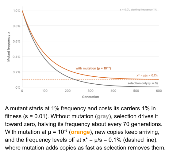
Consider a harmful variant in a haploid population. Let μ denote the mutation rate, and let’s ignore mutations back to the original for now. Let s denote the mutant’s fitness cost. In each generation, mutation adds about μ to the frequency x of the mutant, and selection removes about sx:

$\displaystyle \Delta x = \text{inflow} – \text{outflow} \approx \mu – s x$ $\Delta x = \text{inflow} – \text{outflow} \approx \mu – s x$

The frequency stops changing when the two terms cancel:

$x^* \approx \frac{\mu}{s}$

Imagine a mutation rate of $μ = 10⁻⁵$ . Mildly harmful variants of $s=0.01$ persist at ten times the frequency of more serious mutations of $s=0.1$ . Weaker selection leaves a harmful variant more common. Imperfect copying entails a reservoir of harmful variants. But it also supplies the rare beneficial mutations that selection can spread.

Let’s generalize this to a vector of variant counts n. Selection multiplies each count by its fitness, through a diagonal matrix W. Copying moves offspring between variants, through a matrix Q whose entries $Q_{ij}$ give the probability that parent j will leave an offspring of variant i. One generation is

$n’ = QWn$

This is the replicator–mutator equation (Eigen 1971). Without mutation, Q is the identity matrix and the variant with the largest fitness takes over. With mutation, variants move towards an equilibrium mixture known as a quasispecies (Eigen & Schuster 1979).

Drift

The replicator equation assumes an infinite population. But real populations are finite. Each generation is a sample of the last: offspring are drawn from the parents in proportion to their fitness. Sampling adds noise called drift, which shrinks as N grows. For a variant at frequency x in a population of N haploid individuals, the variance of the change in one generation is

$\displaystyle \operatorname{Var}(\Delta x) = \frac{x(1-x)}{N}$

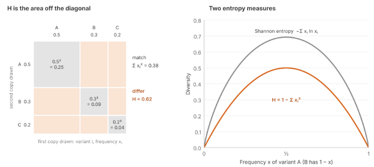
Drift adds noise to frequencies. Ironically, this erodes variation within a population. Let H be the chance that two randomly drawn copies differ:

$H = 1 – \sum_i x_i^2$

Two copies are both variant i with probability $xᵢ²$ , so the sum is the chance they match. In the left image below, H is the area of mismatches off the diagonal.

As a diversity metric, H is known as expected heterozygosity. It is a member of the entropy family, closely related to Shannon entropy.

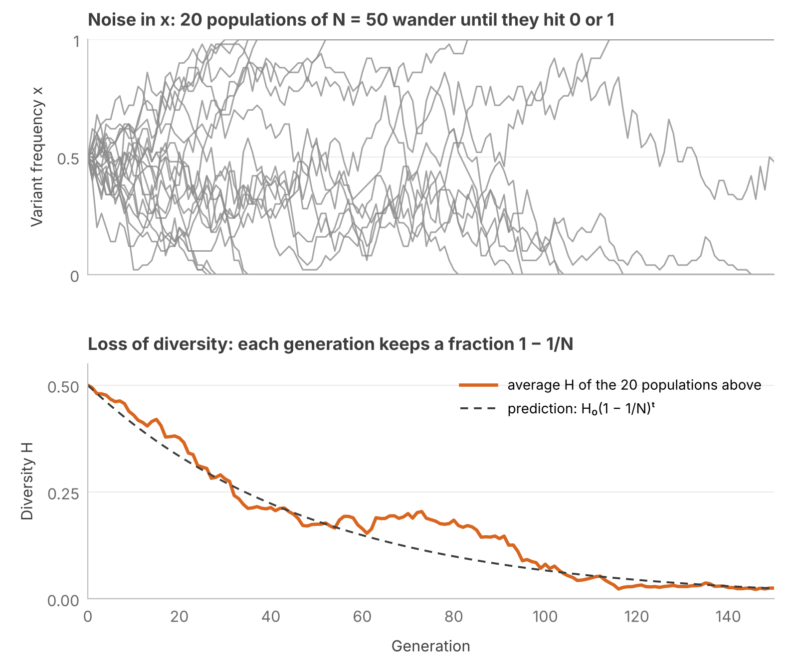
Assume all fitness differences are insignificant. Drift removes diversity in three steps:

x wanders like a fair random walk: its expected step is zero, $\textstyle E[\Delta x | x] = 0$ . Such a walk is called a martingale. From here on, every expectation and variance is conditional on the current frequency x.
0 and 1 are absorbing walls: once a variant is gone, only mutation can bring it back. So every population eventually hits a wall, and none ever leaves one.
Even before any wall is hit, fair steps lower H on average, because H is concave in x: the arch bends downward, so a step down its slope loses more H than an equal step up gains. This is the Jensen gap again, the one that pulls G below A.

With two variants, $H = 2x(1 − x)$ is a parabola, so its Taylor expansion stops at the $\textstyle \Delta x^2$ $Δx²$ term:

$\displaystyle H(x + \Delta x) = H(x) + 2(1-2x)\,\Delta x – 2\,\Delta x^2$

Let $\textstyle H’ = H(x + \Delta x)$ denote the diversity of the next generation. We would like to know its expectation $E[H′]$ : the expected outcome of drift over time.

$\displaystyle E[H’] = H + 2(1-2x)\,E[\Delta x] – 2\,E[\Delta x^2]$

The first expectation is zero, and the second is the step variance:

$\displaystyle E[H’] = H – 2\operatorname{Var}(\Delta x)$

Drift’s step variance then simplifies to:

$\displaystyle \operatorname{Var}(\Delta x) = \frac{x(1-x)}{N} = \frac{H}{2N}$ $\mathrm{Var}(\Delta x) = \frac{x(1-x)}{N} = \frac{H}{2N}$

Putting the pieces together:

$\displaystyle E[H’] = H – \frac{H}{N} = H\left(1 – \frac{1}{N}\right)$

Without a source of new variants, drift pushes finite populations towards uniformity.

In these formulae, we’ve used N as population size. But drift doesn’t care about individuals who don’t reproduce. We require a notion of effective population size Nₑ. How to operationalize it?

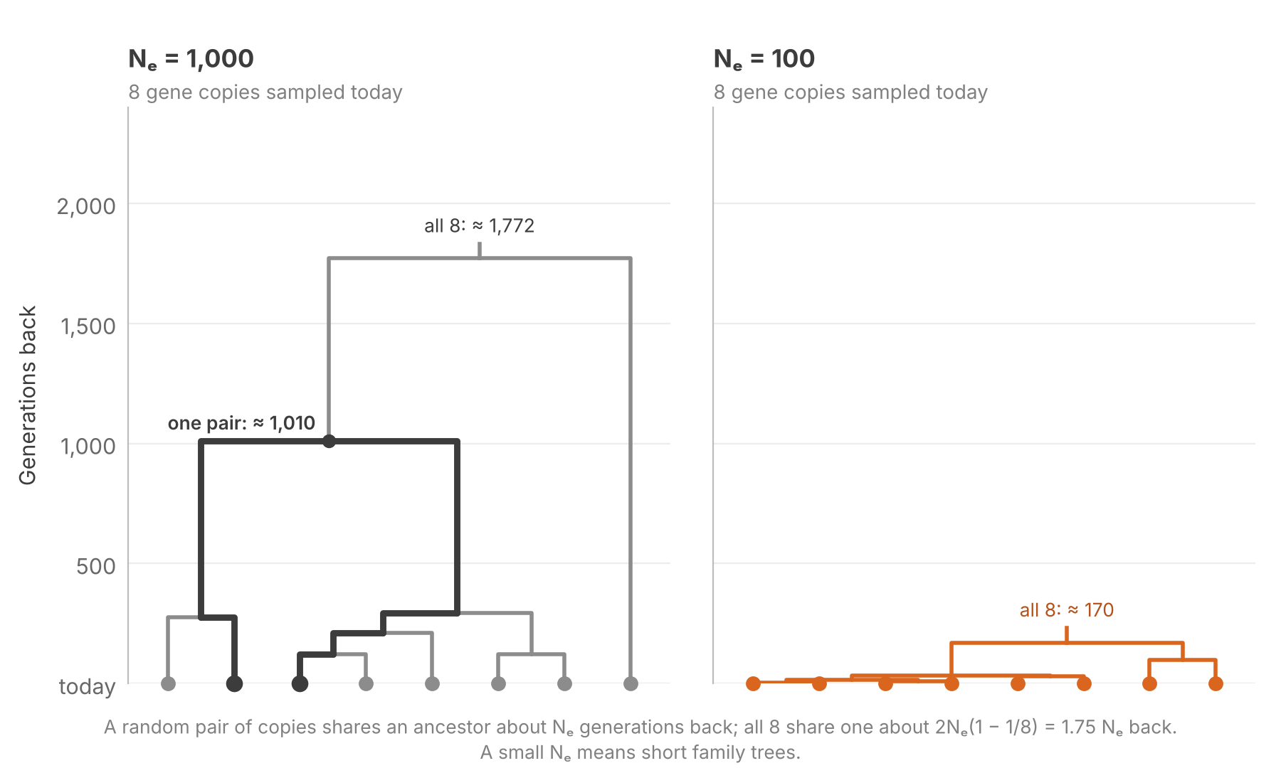
Imagine tracing two gene copies back in time. This backward-facing perspective is called the coalescent (Kingman 1982). In a population of N haploid individuals, two copies share a parent with probability 1/N each generation, so on average they meet in a common ancestor N generations back. Small populations produce shallow family trees.

Let’s start by defining Nₑ as the size of an ideal population with the following property:

$P(\text{two copies share a parent}) = \frac{1}{N_e}$

We can upgrade this abstraction in two ways. First, let $σ²$ be the variance in offspring. In the ideal population, offspring numbers have $σ² = 1$ . But reproductively unequal species can have very large $σ²$ . This increases the probability that two copies trace back to the same parent.

$P(\text{two copies share a parent}) \approx \frac{\sigma^2}{N}$

Some marine species with sweepstakes reproduction have Nₑ thousands of times smaller than their census size (Hedgecock & Pudovkin 2011).

Second, let us countenance changes in population size. Define Nₜ as the census size of parents in generation t, and σₜ² as offspring variance. Two copies share a parent with probability $pₜ = σₜ²/Nₜ$ , and miss with probability $1 − pₜ$ . For two copies to not share a parent, they must miss each generation. Nₑ is the constant effective size that gives the same probability:

$\displaystyle \left(1 – \frac{1}{N_e}\right)^{T} = \prod_{t=1}^{T} \left(1 – p_t\right)$

$\displaystyle T \ln\left(1 – \frac{1}{N_e}\right) = \sum_{t=1}^{T} \ln\left(1 – p_t\right)$

For a small chance p, $\textstyle \ln(1 – p) \approx -p$ , so

$\frac{1}{N_e} \approx \frac{1}{T}\sum_{t=1}^{T} p_t = \frac{1}{T}\sum_{t=1}^{T} \frac{\sigma_t^2}{N_t}$

Nₑ is therefore the harmonic mean of each generation’s Nₜ/σₜ². Population bottlenecks can dominate the harmonic mean. Three generations of 1,000, 1,000 and 10 breeders with σ² = 1 give Nₑ ≈ 29: one crash outweighs many generations of plenty. Humans number in the billions, but our Nₑ is about 10,000 to 20,000 individuals, because for most of our history we were few.

Selection, Drift and Mutation

With our new understanding of drift, let’s reintroduce mutations and selection. Let’s return to an ideal haploid Wright–Fisher population, where $N = N_{e}$ .

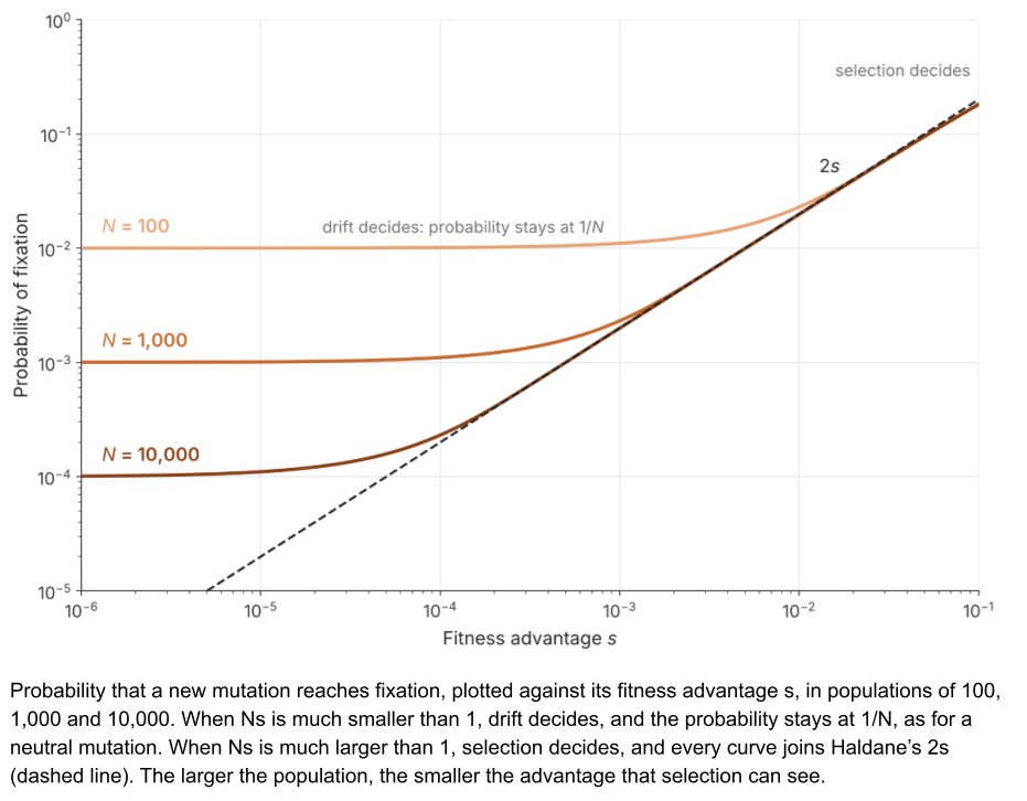
Drift is hardest on new mutations. A single new mutation with fitness advantage s is easy to lose. Haldane (1927) showed that it only reaches fixation with probability about 2s. A mutation that raises fitness by 1% is lost 98% of the time.

Kimura showed that drift and selection operate at different timescales. Selective sweeps have a characteristic timescale of about 1/s generations. Drift needs about Nₑ generations to bring a variant to an absorbing wall. Putting these together:

$\frac{\text{drift time}}{\text{selection time}} \approx \frac{N_e}{1/s} = N_e s$

When $Nₑs$ is much smaller than 1, drift moves the variant before selection can. When it is much larger than 1, selection wins. Kimura’s formula (Kimura 1962) joins the two regimes to capture the probability of fixation:

$P_{\text{fix}} \approx \frac{1 – e^{-2s}}{1 – e^{-2N_e s}}$

Consider two copies.

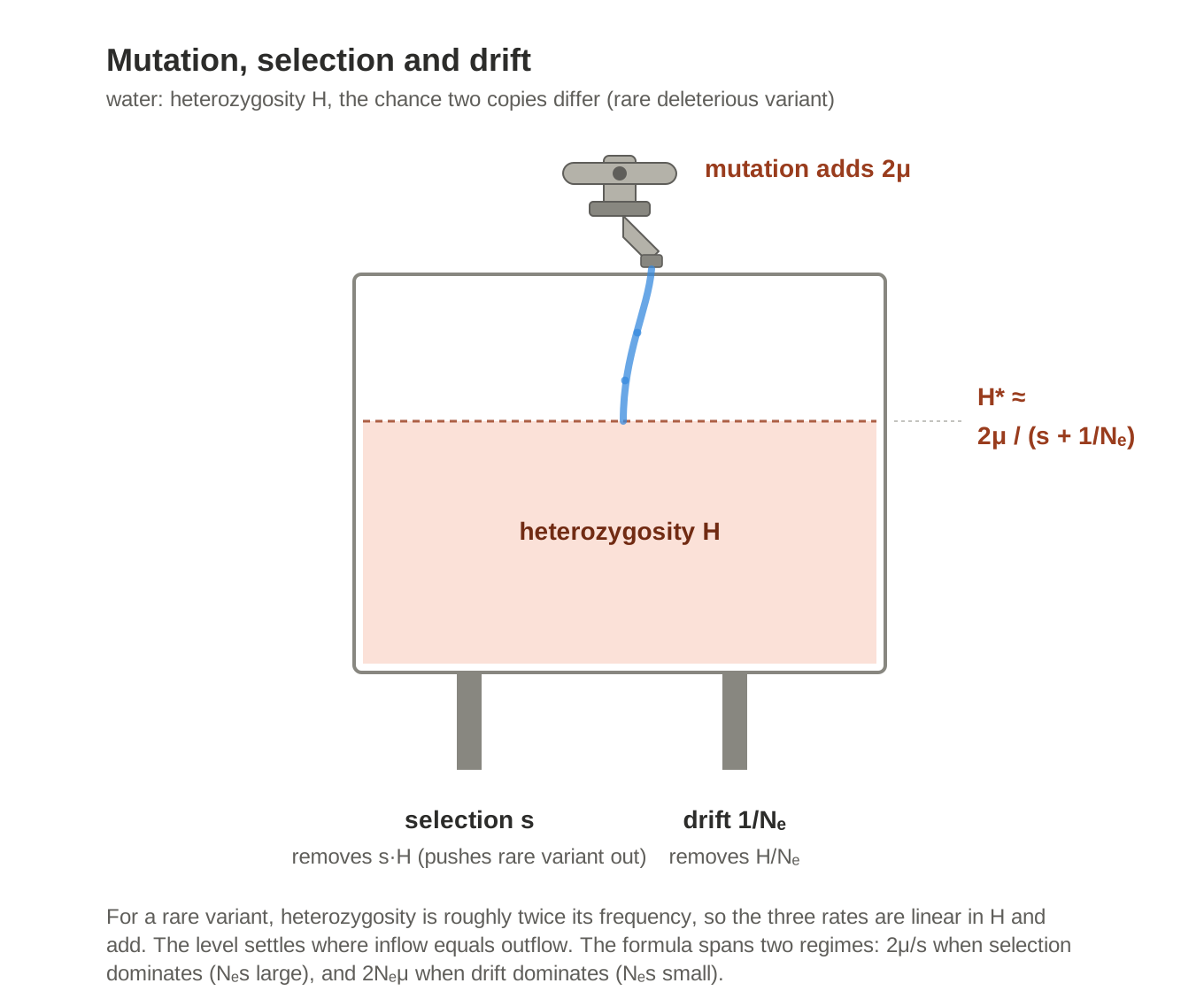
Mutation refills heterozygosity at a rate of 2μ.
A rare deleterious variant is pushed toward extinction, so selection drains its heterozygosity at a rate of s.
Drift drains heterozygosity at a rate of 1/Nₑ.

Let’s set out a heuristic interpolation between the mutation–selection and mutation–drift balance points. Heterozygosity H settles where inflow equals outflow:

$H^* \approx \frac{2\mu}{s + 1/N_e}$

When $Nₑs ≫ 1$ , drift is irrelevant and the mutation–selection balance operates. When $Nₑs ≪ 1$ , selection is irrelevant and the mutation–drift balance operates.

Drift also keeps time. A population of N haploid individuals gains about $Nμ$ new neutral mutations each generation, and each one reaches fixation with a probability equal to its starting frequency, 1/N. The population size cancels:

$k = N\mu \times \frac{1}{N} = \mu$

Neutral substitutions therefore accumulate at the mutation rate, whatever the size of the population (Kimura 1968), and biologists use this molecular clock (Zuckerkandl & Pauling 1965) to date the divergence of lineages from the differences between their sequences.

When beneficial mutations are rare, a population adapts one selective sweep at a time. Each new mutation survives drift with probability about 2s, then spreads along the S-curve of the replicator equation (Gillespie 1984).

Applications

Faced with a new replicator, people first ask its doubling time. But two other questions pertain. Does its fitness fall once it is common, and does it carry a heritable state that can change? Let’s apply these questions to three examples.

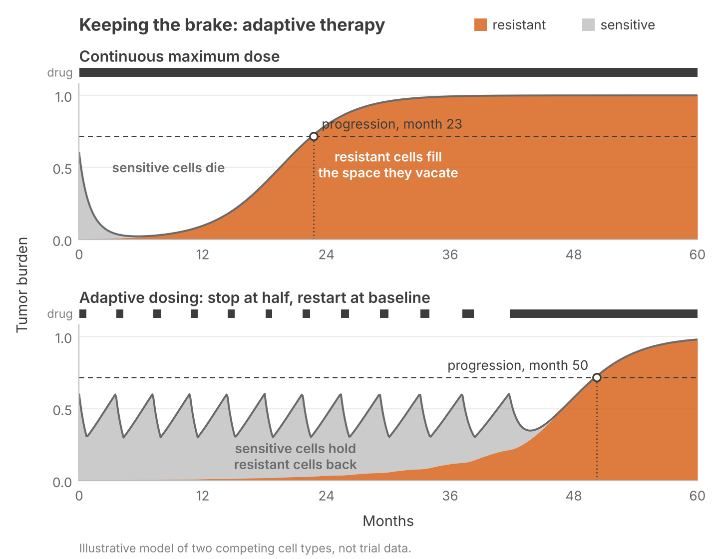
First, drug-sensitive and drug-resistant tumor cells compete for the same nutrients. Treatment at the maximum dose kills the sensitive cells. But this produces a competitive release: it hands the tumor to the resistant cells. Adaptive therapy pauses the drug before the sensitive cells are gone, so they continue to suppress their rivals (Zhang et al. 2017). In a nonrandomized pilot trial of 11 men with metastatic prostate cancer, median time to progression was at least 27 months, compared with about 16.5 months for standard continuous dosing in a large phase III trial.

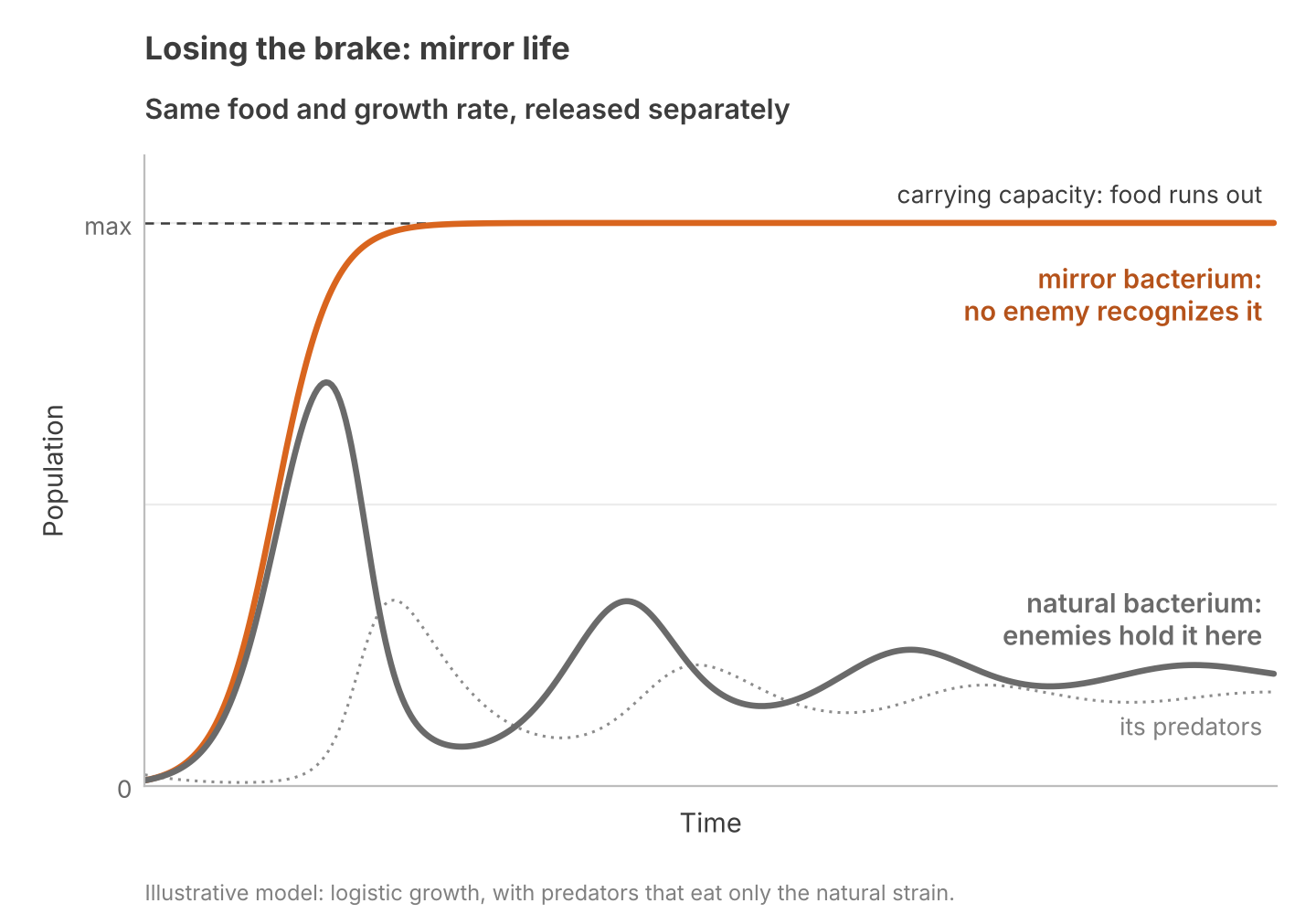
Second, let’s consider mirror life. During abiogenesis and for mysterious reasons, life on Earth became homochiral. Geochemistry produces racemic molecules, with equal proportions of right and left-handed configurations. But proteins use only left-handed amino acids and DNA only right-handed sugars. A mirror bacterium could be built with proteins and nucleic acids of the opposite handedness, and it would likely replicate at similar rates.

Mirror life is dangerous for other reasons. In conventional life, predators hold populations far below the carrying capacity of the environment. But predators recognize their prey by molecular shape, so a mirror bacterium could grow without these constraints (Adamala et al. 2024). Ecologists call this enemy release.

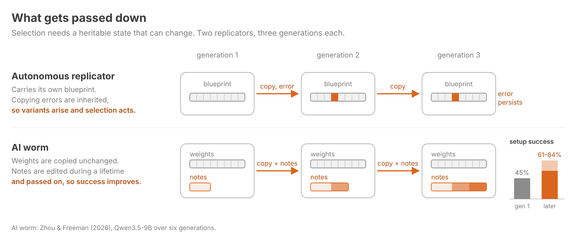
Finally, consider replicating software. Many botnets are spread from a central server, which nanotechnologists call a broadcast architecture (Phoenix & Drexler 2004). For example, Mirai doubled in size every 76 minutes (Antonakakis et al. 2017). But these bots are duplicated exactly, so selection has nothing to act on.

Zhou & Freeman (2026) asked whether open-weight LLMs could spread across consumer devices such as TV boxes and phones. As of October 2026, no such worm exists. In separate experiments, the authors estimated from hardware throughput that a 9B model would take one to two days per replication, and found that when each instance left notes for its successor, inference-setup success rose from 45% in the first generation to 61–84% in later ones. These notes constitute a heritable state.

Doubling time constrains how a replicator starts. Our other questions reveal where it ends.

Relation to Prior Work

In 2015, I wrote three posts which built these intuitions geometrically. Intro to Population Genetics placed each genotype at a location in gene space, so a species is a cluster of points and xᵢ is the fraction sitting at location i. Intro to Natural Selection gave that space a height, fitness, and read selection as uphill motion on the landscape. Fitness Seascapes let the landscape change from place to place and moment to moment, which is just environment-dependent fitness.

Those posts lived in gene space, the space of DNA sequences. This one swaps that for a space of heritable states, which is what the origin of life requires: its replicators range from autocatalytic sets of small molecules to self-copying RNA, none of them DNA.

Wrapping Up

This post relaxed three of the replicator equation’s four assumptions.

Each assumption we relaxed had consequences.

Fitness can change in three ways.
1. Density dependence can keep rivals alive or lock in whichever variant got ahead.
2. Frequency dependence keeps rivals alive.
3. A fluctuating environment can favor variety among one parent’s offspring.
Imperfect copying entails mutation. Mutation is the source of variation needed to keep the engines of selection and drift running.
Finite populations entail drift. Like selection, drift erodes variation. In small populations, drift can overwhelm selection that would win in a larger population.

One assumption held throughout this post: that every individual belongs to exactly one variant. Variant partitions require access to heritable state. But we can measure a giraffe’s neck without knowing which of thousands of alleles shaped it. It would be nice to reason directly about the fitness of phenotypes.

Next time, we will relax this assumption and work with measurements directly. See you then!

References

Adamala et al. (2024). Confronting risks of mirror life.
Antonakakis et al. (2017). Understanding the Mirai botnet.
Botero et al. (2015). Evolutionary tipping points in the capacity to adapt to environmental change.
Chesson (2000). Mechanisms of maintenance of species diversity.
Cohen (1966). Optimizing reproduction in a randomly varying environment.
Cohen (1967). Optimizing reproduction in a randomly varying environment when a correlation may exist between the conditions at the time a choice has to be made and the subsequent outcome.
Eigen (1971). Selforganization of matter and the evolution of biological macromolecules.
Eigen & Schuster (1979). The Hypercycle: A Principle of Natural Self-Organization.
Galloway et al. (2021). Emergence of SARS-CoV-2 B.1.1.7 lineage — United States, December 29, 2020–January 12, 2021.
Gause (1934). The Struggle for Existence.
Gillespie (1984). Molecular evolution over the mutational landscape.
Haldane (1927). A mathematical theory of natural and artificial selection, Part V: Selection and mutation.
Hedgecock & Pudovkin (2011). Sweepstakes reproductive success in highly fecund marine fish and shellfish: a review and commentary.
Hofbauer (1981). On the occurrence of limit cycles in the Volterra–Lotka equation.
Kelly (1956). A new interpretation of information rate.
Kimura (1962). On the probability of fixation of mutant genes in a population.
Kimura (1968). Evolutionary rate at the molecular level.
Kingman (1982). The coalescent.
Lewontin & Cohen (1969). On population growth in a randomly varying environment.
Marshall & Wrangham (2007). Evolutionary consequences of fallback foods.
Maynard Smith (1982). Evolution and the Theory of Games.
Maynard Smith & Price (1973). The logic of animal conflict.
Peters & Gell-Mann (2016). Evaluating gambles using dynamics.
Phoenix & Drexler (2004). Safe exponential manufacturing.
Seger & Brockmann (1987). What is bet-hedging?
Szathmáry & Gladkih (1989). Sub-exponential growth and coexistence of non-enzymatically replicating templates.
Szathmáry (1991). Simple growth laws and selection consequences.
Taylor & Jonker (1978). Evolutionarily stable strategies and game dynamics.
von Kiedrowski (1986). A self-replicating hexadeoxynucleotide.
Zhang et al. (2017). Integrating evolutionary dynamics into treatment of metastatic castrate-resistant prostate cancer.
Zhou & Freeman (2026). AI models may be capable of self-replicating without access to a datacenter.
Zuckerkandl & Pauling (1965). Evolutionary divergence and convergence in proteins.

The Reliability Ratio

October 8, 2026October 10, 2026kevinbinz 2 Comments

Part Of: Machine Learning sequence
Followup To: OLS Estimation via Projection
Content Summary: 4800 words, 24 min read

The Reliability Ratio

A student scores 2 standard deviations (SD) above the mean on an exam, in about the top 2%. A month later she retakes the exam. Even if nothing about her changes, her second exam score will probably be lower. How much lower? One number answers this question: the reliability ( $λ$ ) of the test.

To understand reliability, classical test theory (CTT) splits her score into two steps. Write it as $x = s + n$ . The first step, the signal s, runs from the population mean to the student’s true score: the average she would earn over many sittings. The second step, the noise n, runs from her true score to her observed score.

Let’s imagine each true score is a type. Students of the same type still get different scores, because each sitting draws its own error. Suppose type k has true score $s_k$ and makes up a fraction $p_k$ of the population. Each distribution of types is the normal distribution $\mathcal{N}\big(s_k, \operatorname{Var}(n)\big)$ . The population is their weighted sum:

$f(x) = \sum_k p_k , \mathcal{N}\big(s_k, \operatorname{Var}(n)\big)$

The same distribution of observed scores can come from two different situations. One sitting per student cannot tell the two situations apart.

Because n is independent of s, the two variances add:

$\operatorname{Var}(x) = \operatorname{Var}(s) + \operatorname{Var}(n)$

To see why, square a student’s deviation: $(s+n)^2 = s^2 + 2sn + n^2$ . Average each term over all students. The first gives $Var(s)$ , and the last gives $Var(n)$ . Inside one bell, s is fixed and n averages to zero, so the cross term $2sn$ also averages to zero.

Because the variances add, each one is a share of the whole. The share that comes from true scores is the reliability of the test:

$\text{Reliability: } \lambda = \frac{\operatorname{Var}(s)}{\operatorname{Var}(x)}$

It runs from 0 to 1, and the error share is 1 − λ. In the figure, Var(x) = 1, so λ is 0.8 on the left and 0.2 on the right. So λ describes a test in one population. Give the same test to a narrower population, and Var(s) falls while Var(n) stays the same, so λ falls.

The Coefficient of Determination

Reliability answers a question: how much of the variance in observed scores does the true score predict? Regression answers the same question with the coefficient of determination.

Regress an outcome y on one predictor. The fitted line makes a prediction ŷᵢ for each observation, and the residual $eᵢ = yᵢ − ŷᵢ$ is the error that remains.

A model’s mean squared error (MSE) measures the performance of the model:

$\text{MSE}{\text{model}} = \frac{1}{N}\sum_i (y_i – \hat{y}i)^2 = \frac{1}{N}\sum_i e_i^2$

The coefficient of determination (R²) measures how well the model’s predictions track the outcome. It compares the model’s MSE with a baseline that predicts the mean ȳ for every observation:

$\text{MSE}{\text{base}} = \frac{1}{N}\sum_i (y_i – \bar y)^2 = \operatorname{Var}(y)$

R^2 = 1 – \frac{\text{MSE}{\text{model}}}{\text{MSE}{\text{base}}}

If the model predicts every observation exactly, R² = 1. If it matches the baseline, R² = 0.

Two properties of least squares will be used in this section. First, the residuals average to zero. Second, they are uncorrelated with the predictions.

Given the first property, and the fact that a variable with zero mean has a variance equal to its mean square:

$\text{MSE}{\text{model}} = \frac{1}{N}\sum_i e_i^2 = \operatorname{Var}(e).$

We can now write the coefficient of determination in terms of variances:

$R^2 = 1 – \frac{\operatorname{Var}(e)}{\operatorname{Var}(y)} = \frac{\operatorname{Var}(y) – \operatorname{Var}(e)}{\operatorname{Var}(y)}$

The second property splits the variance of the outcome. Since y = ŷ + e, its variance is,

$\operatorname{Var}(\hat y + e) = \operatorname{Var}(\hat y) + \operatorname{Var}(e) + 2\operatorname{Cov}(\hat y, e)$

The covariance term is zero, so

$\operatorname{Var}(y) = \operatorname{Var}(\hat y) + \operatorname{Var}(e)$

Substitute this into the numerator:

$R^2 = \frac{\operatorname{Var}(\hat y)}{\operatorname{Var}(y)}$

This equation is why R² is also called the explained variance.

In CTT, the noise n has both properties, so x = s + n is a least-squares regression with fit x̂ = s. We cannot run this regression, because true scores are hidden. Its R² still exists, and it is the reliability:

$R^2 = \frac{\operatorname{Var}(\hat x)}{\operatorname{Var}(x)} = \frac{\operatorname{Var}(s)}{\operatorname{Var}(x)} = \lambda$

CTT assumes these properties. In regression, least squares provides them for the training data. On new data, the model can underperform baseline, and R² can be negative.

The Geometry of Variance

OLS Estimation via Projection showed that least squares projects a vector onto the column space of a matrix A. The residual e is perpendicular to that space: $A^\top e = 0$ . The same geometry organizes variance.

Treat each variable as a vector with one entry for each of the N students. Subtract the mean from each entry, and divide each entry by √N. The covariance is an average of products:

$\operatorname{Cov}(u, v) = \frac{1}{N}\sum_{i=1}^{N} (u_i – \bar u)(v_i – \bar v)$

Each vector carries a factor of 1/√N, so their dot product carries 1/N. For these vectors, statistics and geometry are related by the following identities.

$\operatorname{Cov}(u, v) = u \cdot v, \qquad \operatorname{Var}(u) = |u|^2, \qquad \sigma_u = |u|$

The correlation (r) of two variables is the covariance of their standardized versions, $z_u = u/\sigma_u$ and $z_v = v/\sigma_v$ . In vector terms, this divides the dot product by both lengths, which gives the cosine of the angle between the vectors:

$\text{Correlation: } r = \frac{\operatorname{Cov}(u, v)}{\sigma_u \sigma_v} = \operatorname{Cov}(z_u, z_v) = \frac{u \cdot v}{|u|,|v|} = \cos \theta$

Two uncorrelated variables have r = 0 = cos 90°, so they are perpendicular.

Signal and noise are uncorrelated, so they are perpendicular, and $x = s + n$ is the hypotenuse of a right triangle. The legs have lengths $\sigma_s = 4$ and $\sigma_n = 3$ , and the hypotenuse has length $\sigma_x = 5$ . The lengths do not add: 4 + 3 ≠ 5. The areas of the squares on the sides are the variances, and they do add: 16 + 9 = 25. In this geometry, variance additivity is the Pythagorean theorem. Fisher (1918) introduced the term variance because of this additivity.

The split $Var(y) = Var(ŷ) + Var(e)$ in the previous section is the same theorem. The prediction and the residual are uncorrelated, so they are perpendicular. Because the vectors are centered, a regression on one predictor projects the outcome onto the predictor.

For an outcome v and a predictor u, the residual $v − bu$ is perpendicular to u, so $u · (v − bu) = 0$ . Write $b_{v|u}$ for the slope of v on u.

$b_{v|u} = \frac{u \cdot v}{u \cdot u} = \frac{\operatorname{Cov}(u, v)}{\operatorname{Var}(u)}$

The slope is the covariance of the predictor and the outcome, divided by the variance of the predictor. The triangle shows the regression of x on s from the previous section. The residual n is perpendicular to the predictor s, so the fit is s itself, and $b_{x|s} = 1$ .
The side s is adjacent to the angle θ, and x is the hypotenuse, so

r = \cos \theta = \frac{\lvert s \rvert}{\lvert x \rvert} = \frac{\sigma_s}{\sigma_x} = \frac{4}{5} = 0.8

$\lambda = R^2 = \frac{|s|^2}{|x|^2} = \cos^2\theta = r^2 = \frac{16}{25} = 0.64$

The reliability is the squared correlation between true and observed scores. This holds for any regression with one predictor:

$R^2 = \cos^2\theta = r^2$

Regression to the Mean

The slope of y on x is $Cov(x, y)/Var(x)$ . Measure both variables in standard deviations, and the slope becomes r. The slope of x on y is also r. In any units, the two slopes multiply to r²:

$b_{y|x}, b_{x|y} = \frac{\operatorname{Cov}(x,y)}{\operatorname{Var}(x)} \cdot \frac{\operatorname{Cov}(x,y)}{\operatorname{Var}(y)} = r^2$

In standard units, unless the correlation is exact, every prediction is less extreme than its predictor. Galton (1886) found this in human stature. He compared the heights of children with the mean height of their parents and found a slope of about two thirds: parents whose mean height is 3 inches above average have children about 2 inches above average. He called this effect regression towards mediocrity. We now call it regression to the mean.

The slope of about two thirds is measured in inches per inch. It differs from the correlation because parental averages vary less than children’s heights.

Regression to the mean also runs backward in time: tall children have parents who are, on average, less tall than they are. The effect doesn’t require a causal mechanism. It manifests whenever measurements share a signal but also draw independent noise.

When a test is administered twice, for example, the two sittings share a true score and nothing else, so their covariance is Var(s). They also have the same variance, Var(x). So the slope of retest on test and their correlation are both $Var(s)/Var(x) = λ$ .

Galton’s data has the same structure. The mid-parent height is a noisy measure of the parents’ mean additive genetic value: the part of genetic value that children inherit on average. A child inherits that value and draws new noise of its own. So the covariance of child and mid-parent is the variance of the genetic signal, and the slope of child on mid-parent is a reliability ratio. The child’s height varies more than the mid-parent’s, so here only the slope equals this ratio. Quantitative genetics calls this ratio heritability. Under simple genetic assumptions, Galton’s slope of about two thirds measures the heritability of height.

Reliability is the slope of retest on test. It is the component of a result that carries over to the next measurement.

Shrinkage

Recall our student with a strong test score. Regression to the mean says her retest will probably be lower. What is her true score?
The geometry section knew the true score (s) and predicted the observed score (x). It regressed x on s. Our student’s case runs the other way. We know only her observed score, so we regress s on x to estimate her true score.

Independent noise adds nothing to a covariance, so the covariance of the true and observed scores is the variance of the signal:
$\operatorname{Cov}(s, x) = \operatorname{Var}(s)$

A slope is this covariance divided by the variance of the predictor, so only the denominator changes:

$b_{x|s} = \frac{\operatorname{Var}(s)}{\operatorname{Var}(s)} = 1, \qquad b_{s|x} = \frac{\operatorname{Var}(s)}{\operatorname{Var}(x)} = \lambda$

If we know a student’s true score, her observed score averages to that true score. When true scores and errors are normal, no curve does better than the line ŝ = λx. This estimate is called Kelley’s rule. Kelley (1927) derived it in the context of test scores. It is a weighted average of the test score X and the population mean μ:

$\hat{s}_{\text{raw}} = \lambda X + (1-\lambda)\mu$

If the test has high reliability, the estimator trusts the score. Else, it trusts the population mean.

Consider students who achieve a test score of 2 SD. By definition of the normal distribution, many of these students have a true score near 1 SD. So an observed score of 2 SD comes more often from a good student with good luck than from an excellent student with average luck. Consider one of these students. Reliability tells us how much of her lead is skill. With a reliability of 0.8, about 80% of her 2 SD lead is skill, so her best-guess true score is about 1.6 SD.

A Kalman filter (Kalman 1960) tracks a hidden quantity with a current estimate. The estimate’s error has variance P, and each measurement adds noise with variance R. These play the same roles of Var(s) and Var(n) in CTT. The estimate has variance P + R. The filter moves its estimate toward the measurement by a weight K called the gain:

$K = \frac{\operatorname{Var}(\text{true step})}{\operatorname{Var}(\text{measured step})} = \frac{P}{P + R}$

The Kalman filter uses Kelley’s rule, but with the current estimate in place of the population mean. A noisy measurement has a small gain and is largely ignored.

Reliability is also a shrinkage factor. It is the share of an observed lead that we credit to the true score.

Attenuated Slopes

The true scores are often latent, but estimating them can enable downstream predictions. An epidemiologist wants to know how much stroke risk rises with blood pressure. She needs the slope of stroke risk y on each patient’s usual blood pressure s. But she has only one reading x per patient, a noisy measure of s. If she regresses stroke risk on the readings, what slope does she get?

Suppose an outcome depends on the true score, $y = βs + ε$ . The slope we want is $b_{y|s} = \beta$ . True scores are hidden, so we can fit only $b_{y|x}$ , the regression of y on the observed score x = s + n. Write $\lambda_x$ for the reliability of x.

$x = s + n,\quad y = \beta s + \varepsilon,\quad b_{y|x} = \frac{\operatorname{Cov}(y,\ x)}{\operatorname{Var}(x)} = \frac{\operatorname{Cov}(\beta s + \varepsilon,\ s + n)}{\operatorname{Var}(x)}$

If we assume the noise n and the error ε are independent of s and of each other, they add nothing to the covariance:

$\operatorname{Cov}(\beta s + \varepsilon,\ s + n) = \beta\operatorname{Var}(s) + \beta\operatorname{Cov}(s, n) + \operatorname{Cov}(\varepsilon, s) + \operatorname{Cov}(\varepsilon, n) = \beta\operatorname{Var}(s)$

$b_{y|x} = \frac{\operatorname{Cov}(\beta s + \varepsilon,\ s + n)}{\operatorname{Var}(x)} = \beta,\frac{\operatorname{Var}(s)}{\operatorname{Var}(x)} = b_{y|s}, b_{s|x} = \beta\lambda_x$

The slope from a noisy predictor is a product of two factors. The first shrinks the observed score to estimated true score by the reliability. The second factor β carries the true score to the outcome. This process is known as attenuation bias, or regression dilution.

An illustration of the shrinkage. Adding noise to the predictor is visualized as horizontal arrows. The slope of the estimated function flattens.

Her slope from the readings is $\beta\lambda_x$ . For predicting stroke from one reading, this is the best slope she can use. To recover β itself, she divides her slope by $\lambda_x$ , which she can estimate from repeated readings on some of her patients. MacMahon et al. (1990) made this correction in studies of blood pressure and heart disease. The corrected associations with stroke and coronary heart disease were about 60% stronger than the uncorrected ones.

A related effect appears in models trained on many features. Suppose the model also sees a feature z that correlates with the true score s. Then z takes over part of the weight that x loses, even if z has no effect on the outcome. If s is a confounder, epidemiologists call the bias that remains after adjusting for x residual confounding (Phillips & Davey Smith 1991).

Attenuated Correlations

Suppose we score a model against labels from one radiologist. The labels are a noisy measure of the true outcome. Write the radiologist’s label as

$\tilde{y} = y + \delta$

where δ is the radiologist’s error, independent of s, n, and ε. How does label noise change the slope and the correlation?

In the algebra, δ adds nothing to the covariance, so the slope is unchanged:

$b_{\tilde y|x} = \frac{\operatorname{Cov}(y + \delta,\ x)}{\operatorname{Var}(x)} = \frac{\operatorname{Cov}(y,\ x)}{\operatorname{Var}(x)} = b_{y|x}$

But the noisy label does attenuate the correlation. Recall our definitions.

$r_{\text{true}} = \frac{\operatorname{Cov}(s,\ y)}{\sigma_s,\sigma_y}, \qquad r_{\text{observed}} = \frac{\operatorname{Cov}(x,\ \tilde y)}{\sigma_x,\sigma_{\tilde y}}$

\lambda_x = \frac{\mathrm{Var}(s)}{\mathrm{Var}(x)}, \qquad \sqrt{\lambda_x} = \frac{\sigma_s}{\sigma_x}, \qquad \lambda_y = \frac{\mathrm{Var}(y)}{\mathrm{Var}(\tilde{y})}, \qquad \sqrt{\lambda_y} = \frac{\sigma_y}{\sigma_{\tilde y}}

The noises are independent, so the numerators are equal.

$\operatorname{Cov}(x,\ \tilde y) = \operatorname{Cov}(s + n,\ y + \delta) = \operatorname{Cov}(s,\ y)$

Multiply the true correlation by a ratio of standard deviations to get the observed correlation:

r_{\text{true}} \frac{\sigma_s \sigma_y}{\sigma_x \sigma_{\tilde y}} = \frac{\mathrm{Cov}(s, y)}{\sigma_s \sigma_y} \cdot \frac{\sigma_s \sigma_y}{\sigma_x \sigma_{\tilde y}} = \frac{\mathrm{Cov}(x, \tilde y)}{\sigma_x \sigma_{\tilde y}} = r_{\text{observed}}

Both reliability ratios reduce the correlation, so observed correlations are closer to zero than true correlations.

r_{\text{observed}} = r_{\text{true}} \frac{\sigma_s}{\sigma_x} \frac{\sigma_y}{\sigma_{\tilde y}} = r_{\text{true}} {(\lambda_x \lambda_y}^{1/2})

Spearman (1904) named this weakening attenuation. To correct an observed correlation, divide it by $(\lambda_x \lambda_y)^{1/2}$ .

In the figure, the left panel has no noise. In the right panel, each point moves up or down by its noise, and its true score stays the same. The noise averages to zero in each bin, so the orange dots stay on the true line, and the slope stays at 1.5. The correlation falls from 1 to ${\lambda_y}^{1/2} = 0.8$ .

These are the regressions of this post, each with its slope and correlation.

Reliability is also an attenuation factor. A noisy predictor keeps the share λ of a true slope, and each noisy measurement keeps the share √λ of a true correlation.

Estimating Reliability

So far, we have treated the reliability λ as known. In practice, we must estimate it. One score per student cannot provide an estimate, but a second score of the same student can. Since test and retest share the true score and nothing else, we saw that their correlation was λ. More sittings give a better estimate of λ, and their average is a more reliable score.

Suppose each of N students sits the test m times. The score of student i on sitting j, and her average across all sittings are:

$x_{ij} = s_i + n_{ij}, \qquad \bar{x}_i = s_i + \bar{n}_i$

The true score and the errors are independent, so their variances add

$\operatorname{Var}(\bar{x}_i) = \operatorname{Var}(s) + \operatorname{Var}(\bar{n}_i) = \operatorname{Var}(s) + \frac{\operatorname{Var}(n)}{m}$

Across m sittings, the reliability of the average $\lambda_m$ is the share of this variance that comes from the true score.

$\lambda_m = \frac{\operatorname{Var}(s)}{\operatorname{Var}(\bar{x}_i)} = \frac{\operatorname{Var}(s)}{\operatorname{Var}(s) + \operatorname{Var}(n)/m}$

For one sitting, recall the signal share and error share:

$\lambda = \frac{\operatorname{Var}(s)}{\operatorname{Var}(x)} \qquad 1-\lambda = \frac{\operatorname{Var}(n)}{\operatorname{Var}(x)}$

The relationship between reliability of the average and single-sitting reliability is known as the Spearman-Brown formula (Spearman 1910; Brown 1910).

$\lambda_m = \frac{m\lambda}{1 + (m-1)\lambda}$

Repeated sittings also let us estimate the signal and noise variances. The spread of each student’s scores around her own average estimates Var(n). The spread of the student averages around the grand average x̄, the average of all the scores, estimates Var(x̄ᵢ). We write these estimates as σ̂²ₙ and σ̂²ₓ̄:

$\hat{\sigma}^2_n = \frac{1}{N(m-1)} \sum_{i=1}^{N} \sum_{j=1}^{m} \left(x_{ij} – \bar{x}_i\right)^2 \qquad \hat{\sigma}^2_{\bar{x}} = \frac{1}{N-1} \sum_{i=1}^{N} \left(\bar{x}_i – \bar{x}\right)^2$

These divisors differ from the 1/N of earlier sections. Scores sit closer to their own average than to their true mean, so dividing by the number of scores would give too small an estimate. Each divisor counts degrees of freedom: m – 1 inside each of the N students, and N – 1 for the averages.

Replace each variance in the equation for the variance of the average with its estimate, solve for the signal variance, and substitute the estimates into both reliabilities:

$\hat{\sigma}^2_s = \hat{\sigma}^2_{\bar{x}} – \frac{\hat{\sigma}^2_n}{m} \qquad \hat{\lambda} = \frac{\hat{\sigma}^2_s}{\hat{\sigma}^2_s + \hat{\sigma}^2_n} \qquad \hat{\lambda}_m = \frac{\hat{\sigma}^2_s}{\hat{\sigma}^2_s + \hat{\sigma}^2_n / m}$

Thus, the Spearman–Brown formula can be applied to estimate λ and $\lambda_m$ .

This method is the analysis of variance (ANOVA), and Hoyt (1941) used it to estimate reliability. ANOVA states both spreads on the scale of one sitting, as the mean square within (MSW) and the mean square between (MSB).

\text{MSW} = \hat{\sigma}^2_n \qquad \text{MSB} = m \hat{\sigma}^2_{\bar{x}}

More sittings make the noise estimate precise. Only more students make the signal estimate precise, because the spread of the averages has N-1 degrees of freedom. With a reliability of 0.8, a second sitting for every student raises the effective sample size by about 11%, and a second set of students raises it by 100%. Extra sittings pay off only when the averaged score is still noisy or when new students are expensive to recruit.

A retest needs a second sitting. Cronbach’s alpha (Cronbach 1951) estimates reliability from one sitting. Each question acts as a short retest of the same true score. So each covariance between two questions estimates the signal variance, and each question’s variance estimates the variance of one score. The average covariance c over the average variance v then estimates the reliability of one question. This estimate assumes that every question measures the true score equally strongly. The m questions play the role of m sittings, and the total score has the same reliability as their average. So the Spearman–Brown formula gives alpha:

$\alpha = \frac{m,c/v}{1 + (m-1),c/v} = \frac{m,c}{v + (m-1),c}$

Psychometricians use alpha to build tests: they keep the questions that raise alpha and drop the ones that lower it.

The two formulas average over different replications. For reliability of the average, the replications are m sittings of the same test on different days. For alpha, they are the m questions of one sitting. Retest reliability and Cronbach’s alpha can differ for the same test. A more granular analysis of variance explains the divergence. Divide each score into four parts:

Ability (e.g., intelligence)
Day state (e.g., sleep or mood)
Question fit (e.g., having studied these topics)
Leftover (e.g., a lucky guess)

Administering a test again on a different day keeps only ability and question fit. Administering different questions in one sitting retains ability and day state. This approach to variance is further elaborated in generalizability theory (Cronbach et al. 1972).

Hierarchical Models

CTT has two levels: students taking multiple tests (i.e., sittings). A hierarchical model (HM) has two levels, but at a different granularity: groups having multiple members. In HM, each score is an observation of the group mean. Sittings are glossed over as part of the individual variance.

Many of our CTT constructs reappear in HM with new labels.

CTT gives every student the same number of sittings, but HM lets groups differ in size. Let mⱼ be the number of students in school j. A school with 20 students and a school with 2,000 students might each report average test scores, and the score of the former is much noisier. Let τ² denote the variance of the true group scores, and σ² denote the variance of student scores within the school. The Spearman–Brown formula gives the reliability of each school:

$\lambda_j = \frac{\tau^2}{\tau^2 + \sigma^2/m_j}$

The estimate of each group mean is Kelley’s rule, with the grand mean μ in place of the population mean:

$\hat{\theta}_j = \lambda_j,\bar{x}_j + (1-\lambda_j),\mu$

Statisticians call this estimate partial pooling. It is a compromise between no pooling (each school keeps its own score) and complete pooling (every group is estimated with the grand mean). Each estimate θ̂ⱼ depends on τ², σ², and μ, and all three come from every group. So each estimate uses information from the other groups. This is known as borrowing strength.

With equal sizes, one weight scales every average, and the rank order stays the same. With unequal sizes, small groups move further toward the grand mean than large groups, so groups can change rank. Wainer (2007) described a case from education. Small schools were overrepresented among the schools with the highest test scores, and this result encouraged large investments in smaller schools. Small schools were also overrepresented among the schools with the lowest scores.

Wainer named the rule behind this pattern de Moivre’s equation: the error of an average of m observations has standard deviation σ/√m. A small school averages few students, so its average has a large error. Large errors put small schools in both tails. The same rule puts small units in both tails in other domains. The US counties with the highest and the lowest kidney cancer death rates are mostly small rural counties (Gelman & Price 1999). Hospitals that treat few patients have the most extreme death rates (Spiegelhalter 2005). Products with few reviews fill both ends of rating lists. Partial pooling moves these small units toward the grand mean.

In the left panel, all 50 of the most extreme schools have fewer than 100 students. In the right panel, the extremes are now mostly large schools.

Reliability is also a pooling weight. It is the share of its own average that each group keeps.

Reliability and Regularization

Intro to Regularization added a penalty on the size of a model’s weights. With standardized and uncorrelated features, this ridge penalty shrinks each least-squares weight toward zero by a factor with the same form as the reliability ratio (Hastie et al. 2009). An unregularized fit corresponds to perfect reliability, taking the data at face value. Training on inputs with added noise has the same effect as ridge regression for linear models (Bishop 1995), so attenuation is also a form of regularization.

Maximum likelihood estimation (MLE) estimates each mean by its observed value. But noise accumulates, and the estimate vector is too long on average. Stein (1956) showed that for three or more means, the MLE is inadmissible: another estimator has lower expected total squared error for every possible set of true means. The means can be unrelated, which is why the result is called Stein’s paradox. James & Stein (1961) gave such an estimator. It pulls every estimate toward zero by one shared reliability factor: the share of the estimates’ squared size that comes from the true means.

Model selection compares candidate models and keeps the one with the best score. Any score used to make this choice is optimistic. The winner probably had good luck on the scoring data, and its score will probably decrease on fresh data. This phenomenon of selection bias (Cawley & Talbot 2010) is another form of regression to the mean. Bidders in auctions call it the winner’s curse (Capen et al. 1971). Data partitioning creates a retest. An untouched holdout set draws fresh luck, so its score is honest.

Wrapping Up

The reliability λ plays five roles:

References

Bishop (1995). Training with noise is equivalent to Tikhonov regularization.
Brown (1910). Some experimental results in the correlation of mental abilities.
Capen, Clapp & Campbell (1971). Competitive bidding in high-risk situations.
Cawley & Talbot (2010). On over-fitting in model selection and subsequent selection bias in performance evaluation.
Cronbach (1951). Coefficient alpha and the internal structure of tests.
Cronbach et al. (1972). The Dependability of Behavioral Measurements.
Fisher (1918). The correlation between relatives on the supposition of Mendelian inheritance.
Galton (1886). Regression towards mediocrity in hereditary stature.
Gelman & Price (1999). All maps of parameter estimates are misleading.
Hastie, Tibshirani & Friedman (2009). The Elements of Statistical Learning.
Hoyt (1941). Test reliability estimated by analysis of variance.
James & Stein (1961). Estimation with quadratic loss.
Kalman (1960). A new approach to linear filtering and prediction problems.
Kelley (1927). Interpretation of Educational Measurements.
MacMahon et al. (1990). Blood pressure, stroke, and coronary heart disease. Part 1, prolonged differences in blood pressure: prospective observational studies corrected for the regression dilution bias.
Phillips & Davey Smith (1991). How independent are “independent” effects? Relative risk estimation when correlated exposures are measured imprecisely.
Spearman (1904). The proof and measurement of association between two things.
Spearman (1910). Correlation calculated from faulty data.
Spiegelhalter (2005). Funnel plots for comparing institutional performance.
Stein (1956). Inadmissibility of the usual estimator for the mean of a multivariate normal distribution.
Wainer (2007). The most dangerous equation.

Biomass as Congealed Electricity

September 21, 2026September 24, 2026kevinbinz 1 Comment

Part Of: Biology sequence
Followup To: A Portrait of LUCA
Content Summary: 5800 words, 29 min read

Redox Chemistry

Last time, we reconstructed the nature of LUCA, the root at the tree of life. Today, we’re going to be taking a deeper look at how life makes a living: how cells harvest electricity to build more of themselves.

Life requires energy influx. Energy influx creates disequilibria and maintains them against relaxation. Some disequilibria are differences between locations. A temperature gradient, a pressure difference, and a concentration difference across a membrane are spatial disequilibria, and they relax by transport. Other disequilibria are differences between the present state of a system and an equilibrium state it can reach without moving anywhere. A supersaturated solution, a mixture of hydrogen and oxygen, and an activated molecule such as ATP or a thioester each hold a state disequilibrium, and they relax by transformation.

Out of this menu of fourteen options, life runs a state disequilibrium called redox. Oxidation is electron loss, reduction is electron gain (recall the mnemonic OIL RIG). Redox (reduction-oxidation) reactions involve both of these as electron transfer dissipates this disequilibrium.

The remainder of this post will explore how life uses redox, and where these disequilibria come from.

A redox couple is the oxidized and reduced form of the same chemical species. When hydrogen gas (H₂) is oxidized, its bond breaks and it releases two electrons, becoming 2H⁺. When carbon dioxide (CO₂) accepts eight electrons (along with eight protons), it is ultimately reduced to methane (CH₄) and water. A donor-acceptor pairing combines two such half-reactions. We write this pairing as 2H⁺/H₂ → CO₂/CH₄.

Each couple has a characteristic voltage known as the reduction potential (E°′). Strongly negative values indicate a couple that gives electrons up readily; positive values represent willingness to accept. Spontaneous donor-acceptor pairings run from smaller reduction potentials to larger. The potential difference ΔE°′ = E°′(acceptor) − E°′(donor) must be positive. Since 2H⁺/H₂ sits at −0.41 V, and CO₂/CH₄ is −0.24 V (potentials at pH 7 from Thauer et al 1977), a methanogen running from hydrogen gas to carbon dioxide gets ΔE°′ = (-0.24) – (-0.41) = 0.17 V. Actual potentials shift with concentrations, gas pressures, and pH, so the available energy depends on the organism’s conditions.

These relationships are often represented with a redox tower. This is done by sorting couples by reduction potential, and inverting the y-axis. The low reduction potentials (strong donors) sit at the top, and the high values (strong acceptors) are at the bottom. Spontaneous donor-acceptor pairings with positive potential difference can be represented as arrows cascading down the tower. Importantly, the magnitude of the potential difference (arrow length) determines the energy released: ΔG°′ = −nFΔE°′, where n is the number of electrons transferred and F is Faraday’s constant.

Electrochemical Cells

Redox disequilibria relax by transformation: electrons transfer in situ. An electrochemical cell separates the two half-reactions in space, connecting a state disequilibrium (the redox gap) to a spatial one (a voltage across space). Oxidation (electron donation) takes place at the anode, reduction (acceptance) takes place at the cathode. Electrons travel from anode to cathode through a conductor. The accumulating charge differences would quickly squelch the redox reaction. To achieve a cell rather than a capacitor, an electrolyte (e.g., salt solution) carries ionic current between the reaction sites. This closes the circuit and balances charge.

We might distinguish between two forms of cell. In a galvanic cell, the donor-acceptor pairing is spontaneous (exergonic). Galvanic cells convert chemical potential into work. They “discharge the battery.” In an electrolytic cell, the donor-acceptor pairings are non-spontaneous (endergonic). These cells consume work to generate chemical potential. They “charge the battery.”

We will soon learn that biological cells are electrochemical cells. To better contextualize this fact, we first turn to non-biological examples.

Consider the Evans experiment, a single drop of water placed on clean steel. Oxygen reaches the metal fastest near the border of the drop, where the film is thinnest, and slowest at the center. The oxygen-poor center becomes the anode, where iron is oxidized to Fe²⁺ and releases electrons. The oxygen-rich periphery becomes the cathode, where dissolved oxygen accepts those electrons and is reduced to OH⁻. Fe²⁺ and OH⁻ diffuse towards each other and precipitate, producing a characteristic ring of rust. These corrosion processes are ubiquitous because they are exergonic and, on iron, unburdened with a protective oxide film. But here, electron flow is effectively short-circuited through the metal itself. The available Gibbs free energy is dissipated mainly as heat.

This same process can be harnessed to do work. Alessandro Volta opened the short circuit in 1800. His voltaic pile consisted of repeated zinc–electrolyte–copper sandwiches, each forming a galvanic cell. Zinc oxidation releases electrons, which are consumed by a reduction at the copper electrode. Because the electrodes are separate pieces of metal, the electrons cannot pass directly between them. They must travel through an external wire, and anything placed in that path, which we will call the load, can capture part of the redox free-energy drop as useful work.

The pile runs because zinc oxidation is downhill. But many reactions we want run uphill. Aluminum is a prized metal, yet on Earth nearly all of it is bound to oxygen. Smelters convert aluminum oxide (Al₂O₃) into aluminum metal by adding three electrons: Al³⁺ + 3e⁻ → Al. Aluminum is a very weak oxidant, with a −1.66 volt potential. Alumina can be reduced with a stronger reductant. Deville did this in 1854 with sodium metal. But the sodium was difficult to manufacture, and aluminum production was as expensive as silver. The Hall–Héroult process lowered costs by instead supplying reducing power directly from electricity. Alumina is dissolved in molten cryolite, and a large current drives the reduction of Al(III) at the cathode to liquid aluminum while carbon is oxidized at the anode. This reaction is non-spontaneous without an external power source. This is why the industry calls aluminum congealed electricity. The metal is a stock: a reservoir of free energy, filled by one process and drained later by another.

What provides work to an electrolytic cell? A galvanic cell can. Within weeks of Volta’s discovery, Nicholson and Carlisle placed the pile’s wires in water and watched hydrogen and oxygen appear. The voltaic pile supplied the 1.23 volts needed to decompose water. The wire connects driving and driven processes. This wire cannot sustain the reaction when the battery depletes. Both processes must proceed in tandem. In direct coupling, a driving process and a driven process are joined without enough storage to separate their operation in time.

Direct coupling is insufficient when energy inflow and outflow proceed at different times and different rates. Consider an off-grid solar installation. During the day the panels supply electrical work, but a house draws power continuously. This setup is enabled if a stock is placed on the wire. By day, the stock (a battery) is charged in an electrolytic process. But whenever the house needs power, the battery discharges in a galvanic process. In buffered coupling, a stock separates two processes in time. The stock is filled when power is available and depleted when it is needed. A single cell can perform both electrolytic and galvanic roles.

Respiration as a Galvanic Cell

Humans eat food and breathe oxygen. Why? Both are delivered to our cells where electrons are stripped from organic matter and sent down the respiratory chain to oxygen. Cellular respiration is a donor-acceptor pairing. Life runs on redox chemistry.

Consider Cupriavidus necator, a bacterium that strips electrons from hydrogen to give to oxygen. We’ve already seen the electrolytic cell from the Nicholson-Carlisle experiment, which consumed energy to separate water. In 1839, William Grove constructed the reverse. He placed platinum electrodes in separate tubes of hydrogen and oxygen, connected them through an acid, and observed a current. Cupriavidus harvests energy in precisely the same way as Grove’s device: 2H⁺/H₂ against O₂/H₂O. But life utilizes this energy differently, as we will see below.

Respiration occurs in the electron transport chain (ETC). While the modern ETC has many components, for our purposes we consider three. Electrons are passed from the entry enzyme towards the exit enzyme, which function as anode and cathode respectively.

The entry enzyme and the exit enzyme differ across organisms. The quinone pool represents their interface. The entry enzyme (e.g., a membrane-bound hydrogenase) must accept electrons from a redox donor and reduce quinone. Quinone takes the two electrons and, from the inner face, two protons, becoming quinol. The exit enzyme (e.g., quinol oxidase), needs only oxidize quinol. (In mitochondria an extra stage, Complex III and cytochrome c, sits between the pool and the exit enzyme.)

The journey of electrons occurs without a wire. Within the proteins, an electron will tunnel between fixed metal centers, iron-sulfur clusters and hemes, spaced no more than about 14 Å apart (Page et al 1999). Between proteins, the electrons continue their journey hitching a ride on the quinone.

Where does the work go? The ETC enzymes are all embedded in a lipid membrane, which in prokaryotes separates the cytoplasm inside from the periplasm outside. The entry enzyme oxidizes the donor and releases its protons in the periplasm. Quinone is reduced in the membrane and takes its two protons from the cytoplasm. The exit enzyme oxidizes quinol and releases those protons on the periplasm, and reduces the acceptor with further protons drawn from inside. Every pair of electrons that journeys from anode to cathode carries several protons from inside to outside. Redox is a driving process; the proton gradient is a driven process. This coupling of state to spatial disequilibrium is called chemiosmosis.

The gradient has an electrical part, Δψ, and a chemical part, ΔpH, and Mitchell (1961) combined them into a single quantity, the proton-motive force (PMF): Δp = Δψ − 59 mV × ΔpH at 25 °C. In mitochondria and most bacteria Δp is 150 to 220 mV, most of it electrical. That is roughly 15 to 20 kJ per mole of protons, and across a membrane 5 nm thick it is a field of about 4 × 10⁷ V/m, ten times the field at which air breaks down and lightning strikes (Lane 2005). Yet despite its strength, the PMF has limited storage capacity. If proton pumping stops while ATP synthesis continues, the gradient runs down. The PMF therefore serves mainly as the immediate link between driving and driven processes. This is direct coupling.

ETC behavior resembles a voltaic pile. If you connect it to a load (the ATP synthase, which we will meet next), the PMF produces work. But what happens if you remove or disable the ATP synthase? In this open circuit, respiration slows because protons cannot return and Δp rises until the chain stalls against it. Chance and Williams (1955) starved the ATP synthase by withholding ADP. Respiration slowed to a crawl, only recovering when ADP was reintroduced. If the membrane develops a leak, this powerful voltage would be discharged in a short circuit. This is how brown fat warms newborns through a regulated leak channel, UCP1. An uncontrolled leak is more dangerous, thermodynamically equivalent to burning sugar via combustion. A short circuit releases the disequilibrium into waste heat, without powering the ATP-producing load.

The PMF produced by the ETC is only biologically useful if it performs work. That work happens at the ATP synthase. This rotor produces an activated molecule known as adenosine triphosphate (ATP). Thermodynamics favors hydrolysis of its terminal phosphate bond, leading to more stable adenosine diphosphate (ADP). Proton flux turns the synthase rotor, and the rotation forces ADP and phosphate together on the inner face. Three to five protons pass per ATP, depending on the organism. This process holds ATP, relative to ADP and phosphate, some ten orders of magnitude above the level equilibrium would allow.

The ATP stock provides a buffer, but it is small. A human turns their whole ATP stock over within a minute or two, working muscle within seconds. The body regenerates roughly its own mass in ATP each day. ATP is called the energy currency of the cell. In many metabolic processes, ATP is used to enable non-spontaneous reactions by the group transfer mechanism. The terminal phosphate is handed to a substrate, which is lifted into a less stable state, and the endergonic step that follows is paid for by the relaxation of ATP toward ADP. Most endergonic steps in metabolism are paid this way. The rest are paid in reducing power, as we will see shortly.

Biological supply and demand rarely coincide. A plant captures sunlight by day but respires continuously. An animal eats at intervals and works continuously. A bacterium meets its substrate in pulses. Our solar-powered house solved this mismatch with the battery. Cells achieve the same buffered coupling solution with hierarchical storage. Phosphate reserves can become ATP directly. But a cell can dissolve only so much. Any reserve held in solution, like phosphocreatine in muscle, is shallow. Carbon-fuel reserves bypass this constraint by leaving the solution via polymerization (which cuts the particle count dramatically) or phase separation. Carbon-fuel reserves (including glycogen, starch, fat, and PHB) thereby unlock much deeper capacity and can last from hours to months. They rely on metabolic processes to convert their redox disequilibrium back into ATP.

We have sketched how redox disequilibrium is harvested to produce the PMF and ATP. But which molecular species does life harvest?

Modularity and Habitat Colonization

The remarkable fact is that life does not care which span. Animals transfer electrons from organic carbon to oxygen. Prokaryotes can instead use donors and acceptors drawn from minerals, dissolved compounds, and gases. The same ETC (quinone pools, iron-sulfur clusters, a rotary ATP synthase) serves an astonishing diversity of habitats. The entry and exit enzymes are simply swapped. Life most likely began with a single donor-acceptor coupling. But modern life uses modular respiration. Donor and acceptor are configurable; the electron transport chain is largely conserved (Jelen et al 2016).

The voltage gap between an organism’s electron donor and acceptor sets the energy it can extract per electron. Power also requires current: a supply of donor and acceptor in the same place. Because life runs in water, the voltage gap has a ceiling. A substance strong enough to change the oxidation state of water will react with the solvent and cannot reach the organism. Hydrogen gas (E°′ = −0.41 V) is the strongest reductant that accumulates in water, and O₂ (E°′ = +0.82 V) is the strongest oxidant that is both abundant and stable in it. As a stylized fact, the largest redox gap available in water is about 1.2 volts.

But on the Hadean Earth, oxygen was absent in bulk because nothing besides water photolysis produced it. The first bioenergetic revolution was the origin of life itself. The best electron acceptors available (carbon dioxide, -0.24 V; ferric iron, ≈ 0.0 V) sat within 0.5 volts of organic carbon. Limited by donor supply, the anaerobic biosphere could fix ~10¹³ mol C per year, or ~0.1 TW (Crockford et al 2023).

Oxygenic photosynthesis heralded the second bioenergetic revolution. Cyanobacteria pushed electrons from water (+0.82 V) into carbon (-0.43 V). Water is inexhaustible, so primary production rose by an order of magnitude, to ~10¹⁴ mol C per year or ~1 TW. The waste product oxygen eventually accumulated in the atmosphere. Heterotrophs were then able to respire this span in the reverse direction. This second revolution allowed life to harvest near its maximum redox span. Subsequent revolutions had to come from current, by relaxing supply constraints.

But life invaded myriad habitats in the early Earth even before oxygenic photosynthesis. The modularity of respiration allows for life to harvest nearly any form of redox disequilibrium anywhere.

A pair of electrons falling 1.23 V from H₂ to O₂ pays 237 kJ per mole of H₂, while the same pair falling 0.17 V from H₂ to CO₂, the methanogen’s living, pays 33 kJ. Between them lie the denitrifiers, iron reducers, and sulfate reducers. Redox pairings correlate with sediment depth. Oxygen is consumed at the surface, followed by nitrate, manganese, iron, sulfate, then finally CO₂ at the deepest layers (Froelich et al 1979). The biosphere fully occupies the redox tower (Falkowski et al 2008).

Microbiologists have even used gaps in the tower to predict the existence of new organisms. In 1977 Engelbert Broda listed a pairing the tower permitted but no known organism used: ammonium as donor against nitrite as acceptor. He argued that such lithotrophs should exist. They were found in the 1990s (Broda 1977; Strous et al. 1999).

In sum, the biosphere runs galvanic cells to convert redox disequilibria into a stock of ATP. This is energy metabolism. What does a cell buy with it?

The Machinery for Biosynthesis

Life uses this energy to self-replicate, and making more cells requires synthesizing biomass. Energy metabolism finances carbon metabolism.

Let’s review how redox chemistry interacts with organic chemistry. Autotrophs consume CO₂ and convert it into organic matter via carbon fixation. Carbon fixation transfers two electrons at a time from reductants to carbon. Each transfer moves a carbon atom one rung along a ladder. Define L as the total bond order from a carbon to oxygen, nitrogen, or sulfur, with a double bond counting twice. As L decreases, the atom transforms from CO₂ to carboxyl to carbonyl to alcohol to hydrocarbon.

Losing L means reducing carbon. But redox does not uniquely constrain carbon chemistry. For bond formation, what matters is the local distribution of those electrons. An electrophile is an electron-poor atom that accepts electrons to form a bond, while a nucleophile is an electron-rich atom or group that donates it. Carbonyls expose a C=O bond, which is electrophilic. Hydrocarbons and alcohols do not expose this, while carboxylates at L = 3 stabilize theirs through resonance and negative charge.

Biomass is deposited as alcohols and carboxyls, and depleted in carbonyls (Jinich et al 2020). Yet despite avoiding carbonyls, biosynthesis requires their reactivity. Most biosynthesis reactions involve a nucleophilic carbon attacking an (electrophilic) carbonyl. This is the carbonyl paradox.

L tracks the two-electron transfers from reductants. But the formal oxidation state (z) also tracks changes in the carbon skeleton. At a fixed L, every C-C coupling increments z and every C-C cleavage decrements it. Defining the total C-C bond order (n), one arrives at the helpful formula z = 2L – 4 + n. Formal oxidation state ranges from +4 in CO₂ to −4 in methane, and every electron added lowers it.

These are carbon-level metrics. To describe a molecule, we can average the oxidation state of its constituents. Zc denotes the average formal oxidation state of a carbon molecule. Biomass sits in the middle. Bains & Seager (2012) scored ~4300 metabolites across a variety of organisms and found a narrow intermediate band, with the vast bulk of metabolites living near Zc = 0.0. Not every intermediate carbon is a metabolite. But biological intermediates are preferentially stable, with lower Gibbs energy (Jinich et al 2020).

Biomass is deposited as L = 0, 1 or 3. Biomass polarization explains how this is reconciled with Zc = 0. Fatty acids, amino acids, and anabolic carboxylates all have a reduced body around 0 and an oxidized tip at L = 3, with almost no carbon at L = 2. Sugars are the exception.

Why does life build intermediate carbon? It has tremendous combinatorial depth. Bains & Seager (2012) showed that, out of 1.7 million small molecules built from CHNOPS atoms, 95% were at intermediate oxidation state. This matters because useful biochemicals must satisfy many constraints at once. The solution space is sparse. Combinatorial depth makes selection possible.

Intermediate carbon is also stable enough to persist in water. Water is gentle enough that most of carbon’s middle can persist. C–C, C–H, and many C–O bonds can survive long enough for complex molecules to accumulate and undergo selection (Pace 2001). Biomass polarization also helps. At cellular pH a carboxylate carries a negative charge, which keeps it dissolved in water and unable to leak through a membrane. Finally, Jinich et al. (2020) find metabolites more soluble than the nonbiological compounds of the same size that life skips.

Before carbon dioxide can be reduced, it must be activated. Activation has two components:

Kinetic lability lowers the barrier to reaction. Lower barriers often dramatically speed up the rate of reaction.
Thermodynamic driving makes a reaction energetically favorable.

Lability and driving are often correlated, but not always. Kinetic trapping describes a metastable molecule. These products “want” to react thermodynamically, but the activation barrier precludes the reaction at reasonable time frames. Nearly all biomass is kinetically trapped. For example, ATP hydrolysis is strongly favorable, yet it persists in water because the uncatalyzed reaction is slow. Biomass remains loaded, and can be harvested for energy once an enzyme opens the barrier.

Driving does not require a change in oxidation state. A carboxylate is stable, but replacing its oxygen with a better leaving group produces an activated acyl compound such as a thioester or acyl phosphate. The carbon stays at L = 3 throughout.

In metabolism, intermediate carbon passes through the carbonyl hazard zone. It is quickly deactivated in a chemically selective manner. Without that control, abiotic carbon can go awry. In an aldol reaction, two carbonyls enter and one exits, so the reaction can continue indefinitely. The chemistry fans outward. Dehydration gradually pulls the survivors into aromatic rings. The resultant products include tar or insoluble organic matter (IOM). Tar is a dead end. It can burn, but no biological reaction can return it to a set of small molecules.

To convert carbon dioxide to biomass, or vice versa, carbon must first become labile. Anabolism requires three ingredients: a carbon source, an energy currency to activate it, and a reductant currency to attach electrons to it. Consider the Calvin cycle. NADPH is too weak a reductant for a carboxylate, so ATP first converts the carboxylation product, 3-phosphoglycerate, into 1,3-bisphosphoglycerate, which NADPH can reduce. Activation comes first; reduction follows; and the product, glyceraldehyde 3-phosphate, is an aldehyde inside the hazard zone. From there the carbon descends by condensation into the forms we know as biomass.

Catabolism does not simply oxidize biomass either. It must first activate the carbon, by phosphorylation or by attachment to coenzyme A, before the oxidations run. The descent returns far more ATP than the climb cost, and the electrons removed reload the reductant pool. Anabolism and catabolism trace the same loop in opposite directions.

Reductant Carriers

We are ready to return to electrochemistry. Galvanic cells convert redox disequilibria into a stock of ATP. Cells use this energy to fix carbon.

The requirement to reduce carbon is in tension with the modularity of respiration. What if the respiratory substrate is not strong enough to reduce carbon? H₂S sits at −0.27 V, NH₄⁺ at +0.34 V, NO₂⁻ at +0.43 V, and Fe²⁺ at +0.77 V in the acidic water where the best-studied iron oxidizers grow. All of these are far weaker donors than biosynthesis requires. How do these cells reduce carbon uphill?

To address this, life routes biosynthetic electrons through two universal reductant carriers. The nicotinamide cofactors NAD(P)H sit at −0.32 V under standard conditions. Ferredoxin, a small iron-sulfur protein, sits between −0.40 and −0.50 V depending on the organism. Once carbon is activated, NAD(P)H can reduce it, and it serves nearly all biosynthetic reductions. Ferredoxin covers the few steps that need a stronger reductant. After donating electrons to biosynthesis, these carriers return in their oxidized forms and must be reduced again.

A reduction carrier provides other benefits beyond enabling the reduction of carbon. The diversity of respiration enables flexible energy capture. But it would be inefficient to tune thousands of metabolic pathways to many dozens of environmental reductants. The reduction currency provides modularity: an adaptor layer between energy capture and biosynthesis. It also provides regulation. Rather than leaving reductants at the potential and concentration imposed by the local habitat, the cell can maintain its reductant pools at controlled redox states. For example, NAD(P)H potential is ideally suited to keep dangerous carbonyls at low steady-state concentration (Jinich et al 2018).

But how does a cell finance carrier recycling? When the environmental reductant is lower potential than the reductant carriers, carrier recycling doesn’t require energy. Hydrogen-eating autotrophs can produce NADH directly, because hydrogen at nominal conditions sits above NAD on the tower. Heterotrophs can reduce their carriers for free as well. The electrons in organic carbon span a wide range of potentials, and metabolism harvests only the deepest ones.

But what happens when the environmental reductant is weaker than the carrier? In that situation, carrier recycling requires work. This is where life can manifest its metabolism as an electrolytic cell.

The Electrolytic Cell

We met electrolytic cells in industrial reduction of alumina to aluminum. If stronger reductants are unavailable, the smelter can deploy external work, and leave that work embodied in the metal. If no stronger reductants are available to life, it can harness PMF from its galvanic cell to perform carrier recycling. Then biosynthesis drives CO₂ to biomass from the reductant carriers. Biomass is congealed electricity.

When reductant recycling is not free, biology has found two ways to fund it with redox disequilibria.

First, reverse electron transport (RET) can pay from the wire. The PMF can push electrons from the quinone pool to NAD⁺, or from H₂ to ferredoxin. Complex I does this in nitrite and iron oxidizers. Ech does this in methanogens that carry cytochromes.

Second, electron bifurcation also taps energy metabolism, but pays earlier. Bifurcation takes an electron pair from a weak reductant and splits it: one electron falls to a high-potential acceptor, and the energy released pays for lifting the other onto ferredoxin.

Both of these solutions involve a redox disequilibrium powering two loads in parallel: synthesizing energy currency and reductant carriers. Energy metabolism and carbon metabolism compete. But there is another way to synthesize reductants without drawing on a redox disequilibrium.

Light can serve the same purpose. A photosynthetic reaction center absorbs a photon and returns the electron at a lower potential than it received. The photon raises the electron by more than one volt, but part of that energy is spent to make the reaction irreversible. The resultant voltage gain (about 0.5 volts) subsidizes carrier recycling. A chemotroph needs an environmental reductant above its carriers on the tower, or it pays for the lift with bifurcation or RET. But an anoxygenic phototroph can use an environmental reductant that is 0.5 volts weaker, because light pays for that part of the lift.

Two families of reaction centers exist.

Purple bacteria carry the type II reaction center, which deposits its electron in the quinone pool. The electron travels through the ETC cyclically, and produces PMF. Quinol is a weaker reductant than NADH, so reductant recycling must use RET. The purple bacterium converts PMF into reductant.

Green sulfur bacteria carry the type I reaction center, which deposits its electron in ferredoxin. Light pays for reductant recycling directly. Electrons reach the reaction center through the ETC, making PMF along the way. They come from the environmental reductant, or from ferredoxin sent back around the loop. The green sulfur bacterium spends reductant to make PMF, the reverse of the purple bacterium.

Light arrives by day, but energy expenditure is continuous. Every phototroph relies on carbon-based storage to bridge the gap. Bacteria use glycogen; plants use starch. The stock is filled by electrolytic anabolism by day, and drained by galvanic catabolism by night. The structure mirrors the solar-power battery bank: two direct couplings separated in time by a stock.

Oxygenic photosynthesis wired both reaction centers in series. The type II center moves electrons from water to the quinone pool. Their descent through the ETC produces energy. The type I center lifts the electrons into a ferredoxin carrier. These photons together pay the whole 1.25 volt span. This was the second bioenergetic revolution.

To sum up, galvanic and electrolytic circuits can coexist. The galvanic circuit harvests the environmental redox gradient as PMF. The electrolytic circuit uses PMF to lift electrons onto the carriers, to enable biosynthesis. A nitrite oxidizer runs both circuits continuously. A phototroph decouples galvanic and electrolytic circuits, with carbon-based storage as the “battery” stock in between.

One question remains. If life harvests redox gradients, what creates the gradients in the first place?

A Planet-Sized Battery

The battery existed before life learned to tap it. The Earth is a planet-sized redox battery (Smith & Morowitz 2016). Its anode is the mantle, rich in ferrous iron. Its cathode is the ocean and atmosphere, rich in carbon dioxide. The resultant redox span from H₂ to CO₂ is 0.2 volts. LUCA tapped this battery first. Plug-and-play respiration came later.

The atmosphere was birthed from volcanic degassing. This process built an atmosphere of oxidized volatiles H₂O, CO₂, N₂, and SO₂. Photodissociation further oxidized the planetary cathode. Ultraviolet light breaks down water in the stratosphere. Hydrogen is prone to escape into the exosphere. The remaining oxygen is electron-hungry, oxidizing whatever it meets. Escaping hydrogen oxidizes our surface (Catling et al 2001). On Earth the process is slow, because the tropopause cold trap freezes water out before it reaches the stratosphere (Catling & Kasting 2017). Venus had no such trap, and photodissociation cost it an ocean (Kasting & Pollack 1983).

The mantle is rich with ultramafic rock, with a great deal of ferrous iron in olivine and pyroxene. Ferrous iron (Fe²⁺) holds one electron more than ferric iron (Fe³⁺), and loves to shed electrons. Serpentinization occurs when seawater reaches this rock. Ferrous iron gives its electron to water, ferric iron is left behind in magnetite and serpentine, and the electron leaves as H₂. H₂ carries the mantle’s reducing power, bringing the planetary anode up into the ocean.

The two terminals do not discharge spontaneously. 4H₂ + CO₂ → CH₄ + 2H₂O is kinetically trapped. The reaction needs a catalyst. Life bridges the gap.

Other planets have iron and water, and some have freed oxygen by photodissociation. But corrosion usually stops. As the surface rusts, the electron-rich iron below becomes blocked. Current persists where fresh rock continues to meet water. On Earth, plate tectonics exposes fresh ultramafic rock at ridges, and subducts oxidized crust. But tectonics is not a hard requirement. Enceladus produces redox disequilibria from a porous core repeatedly damaged from tidal forces (Waite et al. 2017).

Modern serpentinization yields ~10¹² mol of H₂ per year (Cannat et al. 2010; Worman et al. 2016). At 0.2 volts that is ~1.2 GW of chemical power. This planetary battery may have generated enough power to spark the first bioenergetic revolution (Russell et al. 2010).

Until next time.

References

Bains & Seager (2012). A combinatorial approach to biochemical space: description and application to the redox distribution of metabolism.
Broda (1977). Two kinds of lithotrophs missing in nature.
Cannat et al (2010). Serpentinization and associated hydrogen and methane fluxes at slow spreading ridges.
Catling & Kasting (2017). Atmospheric Evolution on Inhabited and Lifeless Worlds.
Catling et al (2001). Biogenic methane, hydrogen escape, and the irreversible oxidation of early Earth.
Chance & Williams (1955). Respiratory enzymes in oxidative phosphorylation. III. The steady state.
Crockford et al (2023). The geologic history of primary productivity.
Falkowski et al (2008). The microbial engines that drive Earth’s biogeochemical cycles.
Froelich et al (1979). Early oxidation of organic matter in pelagic sediments of the eastern equatorial Atlantic: suboxic diagenesis.
Jelen et al (2016). The role of microbial electron transfer in the coevolution of the biosphere and geosphere.
Jinich et al (2018). Quantum chemistry reveals thermodynamic principles of redox biochemistry.
Jinich et al (2020). A thermodynamic atlas of carbon redox chemical space.
Kasting & Pollack (1983). Loss of water from Venus. I. Hydrodynamic escape of hydrogen.
Lane (2005). Power, Sex, Suicide: Mitochondria and the Meaning of Life.
Mitchell (1961). Coupling of phosphorylation to electron and hydrogen transfer by a chemi-osmotic type of mechanism.
Pace (2001). The universal nature of biochemistry.
Page et al (1999). Natural engineering principles of electron tunnelling in biological oxidation–reduction.
Russell et al (2010). Serpentinization as a source of energy at the origin of life.
Smith & Morowitz (2016). The Origin and Nature of Life on Earth: The Emergence of the Fourth Geosphere.
Strous et al (1999). Missing lithotroph identified as new planctomycete.
Thauer et al (1977). Energy conservation in chemotrophic anaerobic bacteria.
Waite et al (2017). Cassini finds molecular hydrogen in the Enceladus plume: evidence for hydrothermal processes.
Worman et al (2016). Global rate and distribution of H₂ gas produced by serpentinization within oceanic lithosphere.

Life’s First Ratchet

August 17, 2026August 17, 2026kevinbinz Leave a comment

Part Of: Biology sequence
Followup To: A Portrait of LUCA
Content Summary: 4000 words, 20 min read

Cutting the Knot

Abiotic chemistry is leaky. Sugars brown into tar. Nucleic acid hydrolyzes in warm water on a timescale of days to weeks. Practically anything soluble diffuses away. Whatever complexity chemistry builds is temporary. To achieve LUCA, chemistry needed a ratchet.

The natural place to look for that ratchet is LUCA’s own subsystems, but they depend on one another. Genes prescribe proteins, yet cannot be expressed without proteins to transcribe and repair them. Metabolism supplies the materials for both, yet runs on protein catalysts that genes encode. Asking which came first is really asking which subsystem supplied the first ratchet.

This Gordian knot is a question of functional priority. There are two ways to cut it.

One answer sees the first ratchet in nucleic acid. A system that can copy information can preserve innovation. This is the genetics-first tradition.

The other sees it in metabolism. A network that captures free energy can maintain its own organization and generate the building blocks heredity would later need. This is the metabolism-first tradition.

The RNA World

Let’s set metabolism aside for a moment. Among the three biopolymers of the central dogma – DNA, RNA, and modern coded proteins – which came first? On this smaller question, the scientific community has achieved consensus. Metabolism-first and genetic-first camps agree: RNA came first.

RNA is the answer because it can do both jobs. RNA stores information in its nucleotide sequence, like DNA. But it also folds itself into structures that catalyze chemical reactions, like proteins. The discovery of self-splicing introns revealed that RNA can act as a catalyst (Kruger et al. 1982). Most modern biological catalysts are protein enzymes. RNA catalysts are called ribozymes. The universal coenzymes hint at the same history. NAD, FAD, coenzyme A, and SAM are all built on nucleotide scaffolds, which White (1976) read as molecular fossils of an RNA-based metabolism.

The ribosome is the engine of the genetic code. Remarkably, we are able to reconstruct its development at the atomic resolution. The oldest part of the ribosome, its center known as the peptidyl transferase center (PTC), contains no proteins at all. Its catalytic heart is entirely RNA. The ribosome is a ribozyme (Nissen et al. 2000).

Other genetic polymers could, in principle, have preceded RNA. One genetic system could also have replaced another while preserving the basic function of heredity, a process sometimes called genetic takeover (Hud et al. 2013). But for now, in the name of parsimony, we will assume the first genetic ratchet was RNA.

Why is protein-first no longer an active research tradition? Amino acids and short peptides may well predate RNA. But RNA apparently precedes modern coded proteins. The RNA World constitutes major progress in cutting the knot. The RNA world is silent on the order of metabolism. This is the residue.

The genetics-first solution advocates a strong version of the RNA World: genetic heredity precedes the emergence of metabolism. Natural selection then improves the chemical system around the replicator. No one questions the capacity of nucleic acids to build and retain complexity. The burden is to show how geochemistry alone can birth such a wondrous digital inheritance.

The metabolism-first tradition holds that metabolism existed before RNA, and therefore before genetically encoded proteins. A non-enzymatic protometabolism must exist first. This school fully accepts digital inheritance. But it proposes that protometabolism served as the first ratchet. Geochemistry is thus less burdened. The burden here is twofold: to show that non-enzymatic protometabolism is viable, and to show that a mere reaction network can preserve innovation without genes. We take up the second question in a later post.

Let us explore the viability of specific genetics-first and metabolism-first theories. These are grounded in specific habitats. But before we search for the Geography of Genesis, we must first understand what success looks like. Designing such a rubric takes us back to first principles. We begin with thermodynamics.

Life as a Dissipative Structure

Free energy is the part of energy that can do work. The second law of thermodynamics says that energy tends to spread out. Hot objects cool, gases mix, and chemical gradients become weak.

A closed system does not exchange matter with its surroundings. Without a continuing source of usable energy, its chemical differences decay toward equilibrium. As a system approaches equilibrium, free energy is dissipated, often as heat, and less remains available to do useful work.

Life manifests tremendous complexity and order. In What Is Life?, Erwin Schrödinger explained that life is not a closed system. An open system can exchange energy and matter, so an external process can maintain nonequilibrium conditions. Life exists in an open system. It consumes external energy and matter, then releases heat and waste. Life keeps local order while disorder increases in its surroundings.

The chemist Ilya Prigogine developed the idea of dissipative structures. These structures import free energy from their environment. They maintain local order by using this energy and releasing heat and waste into their surroundings. When the flow stops, the structure usually weakens or disappears.

Dissipative structures occur at many scales. Examples include convection cells, flames, chemical oscillations, hurricanes, and living organisms. For the origin environments we will consider, two energy sources matter most: sunlight and geological activity.

Our first requirement is sustained free-energy flux. The Garden of Eden must feature continuous (or at least recurrent) throughput sufficient to maintain far-from-equilibrium chemistry.

Chemical Selectivity

Free energy flux can drive useful reactions. It can also drive thousands of useless ones.

In organic chemistry, a small set of reactive molecules can combine in many different ways. Each new product can then react with the original molecules or with other products. The number of possible pathways can grow rapidly. Researchers call this a combinatorial explosion.

Scientific experiments (e.g., Miller Urey) and natural phenomena (e.g., carbonaceous chondrites) both tend to produce tar: complex mixtures that are difficult to separate or even characterize.

The formose reaction gives another example. Recall that ribonucleic acid (RNA) uses one particular sugar: ribose. Under alkaline conditions, formaldehyde produces dozens of different sugars and related compounds, while ribose appears as only one component of the diverse products. As the reaction continues, useful products can disappear into still more complex chemistry.

Life is different. Biology uses an extraordinarily restricted region of chemical space. About 500 naturally occurring amino acids have been identified, but the standard genetic code uses only 20 of these to build proteins. The same organizing principle appears in metabolism. Smith and Morowitz (2004) identify eleven TCA-cycle carboxylic acids as a universal anabolic core, from which the major pathways of biosynthesis branch. In their formulation, lipids, sugars, amino acids, nucleotides, and other major classes of biomolecules are ultimately built outward from this small conserved core.

A biochemical environment must channel significant flux toward its target products, while limiting competing reactions. This is a second requirement for Eden: chemical selectivity.

For genetics-first, this requirement must be met before selection can start. A nucleic acid is a monument of chemical selectivity: one sugar among dozens, a few bases among many, the correct linkage among several. The environment must achieve that discrimination unaided. Genetics-first chemistry therefore requires prebiotic mechanisms that narrow the product distributions.

Metabolism-first theories propose another possibility. Positive feedback reactions (aka autocatalysis) can deliver selectivity without a special environment. But it only works if the network reinforces a restricted set of productive reactions, rather than amplifying chemical clutter. We will explore this topic in more detail in a followup post.

Deriving the Rubric

We can say more. Chemical principles allow us to derive five additional requirements.

Provenance. The required feedstocks and catalysts must arise or arrive naturally.
Reactant Concentration. Feedstocks must reach concentrations high enough for useful reactions.
Material Flux. Fresh material and free energy must continue to enter, while waste leaves and spent material is removed, reactivated, or recycled.
Product Retention. Useful products must also remain close by long enough to interact again, rather than immediately dispersing into the environment.
Net Production. Eden must not only produce these target products. It must produce them faster than it destroys them. We require net production.

Material flux and product retention are in creative tension. Eden must eject waste while selectively retaining useful products.

The above concerns single reactions. But theories of abiogenesis rely on many processes.

Suppose one reaction requires acidic conditions, another alkaline conditions. Or one may require intense ultraviolet radiation, while another important product is rapidly destroyed by the same radiation. A theory may need to confine different reactions to different microenvironments. Such conflicts do not make a pathway impossible, but they do require that these microenvironments exchange products in a realistic way. This is the requirement for condition compatibility.

It is not enough to demonstrate each reaction separately in a laboratory. Products of one step must naturally reach the next without artificial purification, isolation, or reagent replacement. This is the requirement for process continuity.

A favorable environment is of little use if it disappears before cumulative organization can develop. The environment must persist or recur often enough to provide continuity across time. Our last requirement is habitat persistence.

These requirements are universal. But genetics-first and metabolism-first theories also generate idiosyncratic requirements. Let’s examine each in turn.

Building Nucleic Acid

Genetics-first demands a specific product. Geochemistry must synthesize a nucleotide. Every nucleotide brings together a sugar (ribose), a nitrogenous base, and a phosphate group into a single large molecule:

Carbon, hydrogen, and oxygen are readily available in many geological habitats. Nucleotides also require nitrogen and phosphorus, and these present new challenges for genetics-first models.

Most environmental nitrogen is molecular nitrogen, N₂. The strong triple bond in N₂ makes it unusually unreactive. Before nucleotide synthesis can begin, some process must supply fixed nitrogen in a reactive form. Nitrogen fixation is one way to make it more reactive (Mateo-Marti et al. 2019). Similarly, phosphorus is present in rocks, but much of it occurs in minerals with low solubility. In water containing calcium, dissolved phosphate is quickly locked away into minerals. Many prebiotic reactions, meanwhile, require phosphate concentrations far above those found in ordinary natural waters. This is the phosphate problem (Toner and Catling 2020). Together, these problems generate two requirements. A genetics-first theory requires bioavailable nitrogen and phosphate.

Of course, individual nucleotides aren’t enough. They must come together as long strands of nucleic acid.

RNA polymerization occurs through a condensation reaction. But condensation polymerization is disfavored in water. The equilibrium instead favors the reverse reaction, hydrolysis. Joining nucleotides into a chain therefore requires an input of free energy (Yadav et al. 2020). Monomer activation denotes the requirement to store or couple this free energy so that phosphodiester-bond formation can proceed.

Providing free energy is not enough. Polymerization also requires high efficiency. A 45-nucleotide polymer requires 44 bond-forming steps. At each step, the chain can degrade. Even modest inefficiency therefore compounds across the chain. Polymer elongation denotes the requirement for bond formation to be efficient enough to produce functional-length polymers.

Towards a Replicator

We’ve established a long RNA polymer. Next, it must copy itself.

Natural selection cannot act on sequence information until polymers are long enough for different sequences to produce different functional structures. Very short oligomers have limited capacity to fold into complex three-dimensional forms.

We do not know a strict minimum length for a useful hereditary polymer. But Gianni et al. (2026) provide an important empirical benchmark. They discovered QT45, a polymerase ribozyme only 45 nucleotides long. QT45 can catalyze synthesis of both its own sequence and its complementary strand.

Recall that nucleotides attach to their complements via Watson-Crick pair bonds. These bound duplexes are very stable. This stability assists during the replication, but presents a problem afterwards. If the strands remain bound, neither is available as a template for the next generation. This is the strand inhibition problem. For replication to persist, the resulting duplex must separate without damaging the sequence. Template reset denotes this requirement.

A catalyst that helps every molecule around it, freeloaders included, gains nothing from its own innovation. Some mechanism must couple products to their producers: what a system makes must preferentially benefit that system. Compartments are the obvious mechanism, but mineral pores, surfaces, and reaction-diffusion gradients are candidates too. As we will see in a later post, this requirement bites both camps, and selection will demand a sharper version of it.

So ends our discussion of genetics-first. Now we turn to metabolism-first theories.

The Twin Engines of Protometabolism

Genetics-first requires a specific deliverable: self-replicating RNA. Where is the analogue for metabolism-first? Which seeds accreted the fantastic complexity of modern metabolism?

Metabolic networks are not tangled webs. Their architecture is hierarchically modular: tightly linked modules nest within larger modules, all organized around a small connective core (Ravasz et al. 2002). Architectures like this arise when networks expand by attachment, each new pathway bolting onto machinery that already exists. And once a dozen downstream pathways depend on an upstream reaction, that reaction is frozen in place; changing it breaks everything built on top. Wimsatt (2007) calls this generative entrenchment. Entrenchment gives the network a readable stratigraphy. Deeply embedded core chemistry should tend to be older than dependent peripheral pathways. We will meet the same logic again when we explore the ribosome’s history from its onion-like layers.

All living things rely on energy metabolism to fuel themselves and anabolism to build up complex organics. The differences reside where the carbon comes from. Autotrophs use carbon fixation to build biomass from inorganic carbon such as CO2. Heterotrophs obtain reduced carbon from the environment, and rely on catabolism to break down the complex organics in their diet.

The modern biosphere rests on an autotrophic foundation. Nearly all carbon enters through the fixation of CO2. Life does not depend significantly on extraterrestrial, atmospherically or geologically produced organics. But on the Hadean Earth, impact delivery supplied organics at a far higher rate. Oparin and Haldane’s original vision of primordial soup presumed a heterotrophic origin. So which was it? Did the first life eat chondrites or fix carbon?

Two converging lines of evidence suggest fixation. The first comes from genes and energetics. Weiss et al. (2016) traced 355 gene families back to LUCA and recovered the profile of an anaerobic, H2-dependent autotroph. Phylogenetic reconstructions are often contested. But Wimmer et al. (2021) computed the thermodynamics of LUCA’s ~400 core reactions and found that roughly 96% run exergonically under H2-rich anoxic conditions. The genes describe an autotroph, and the metabolism they encode fits an autotroph’s environment.

The second line of evidence applies our stratigraphy. Catabolism sits at the periphery. Major catabolic pathways characteristically converge on the universal anabolic core. Moreover, the substrates it digests are sugars, lipids, and proteins: the characteristic products of anabolism (Schönheit, Buckel & Martin 2016). The enzyme record concurs. The ancestral fructose-bisphosphate enzyme of archaea is locked into the gluconeogenic direction, marking glycolysis as a later retrofit (Say & Fuchs 2010).

Taken together, these suggest that anabolism came first. The first life was likely autotrophic.

Carbon fixation places specific requirements on the environment. It requires both CO2 and a continuous electron supply. Candidate electron donors (reductants) include H2, Fe(II), and H2S. Reductant and carbon co-delivery denotes the requirement that electron donors and inorganic carbon arrive together, continuously, at rates sufficient to sustain fixation.

Anabolic metabolism synthesizes thousands of biological molecules. The stratigraphy points inward: the oldest chemistry of all should sit at the very center of the network. Smith and Morowitz (2004) identify it. Eleven carboxylic acids form a universal anabolic core.

With a handful of glycine-related exceptions, all biosynthesis radiates from five of these acids. Acetate seeds the lipids; pyruvate the sugars and the alanine-family amino acids; oxaloacetate the aspartate family, and through aspartate the pyrimidines; α-ketoglutarate the glutamate family; succinyl-CoA the pyrroles. (Purines are the untidy exception, assembled from glycine, aspartate, glutamine, and the same C1 chemistry owned by the WL pathway) These are the pillars of anabolic metabolism.

The entire biosphere uses seven carbon fixation pathways (CBB, rTCA, WL, 3-HP, 3-HP/4-HB, DC/4-HB, and roTCA). Which of these was used by LUCA?

You may recall learning about the tricarboxylic acid (TCA) cycle (aka Krebs cycle) at school. In modern organisms, this cycle is catabolic. For decades that was its only known direction. But Evans et al (1966) and Shiba et al (1985) discovered it also runs in the reverse direction. This rTCA cycle is an autotrophic engine of carbon fixation. The eleven carboxylic acids are precisely the universal anabolic core. It is a strong candidate for the seed of protometabolism.

Several steps of any fixation pathway are endergonic (thermodynamically dysfavored) under ordinary conditions. Modern cells pay for these steps with ATP hydrolysis. A protometabolism has no ATP. The environment itself must pay. Thermodynamic drive denotes the requirement that environmental chemistry makes the overall pathway favorable without modern energy currencies like ATP.

We have identified the rTCA cycle by reading the network’s stratigraphy. Comparative biology provides another glimpse. Consider organisms that are anaerobic and chemoautotrophic. In archaea, these are the methanogens; in bacteria the acetogens. What do they have in common?

Both methanogens and acetogens rely on the Wood-Ljungdahl (WL) pathway (aka acetyl-CoA pathway). WL is in fact the only carbon-fixation pathway found in both bacteria and archaea. Weiss et al (2016) place WL in LUCA itself. WL is also thermodynamically unique. Every other fixation pathway runs uphill and is financed with ATP. The Calvin cycle spends roughly nine ATP per pyruvate; rTCA is among the cheapest. WL runs downhill. Under anoxic conditions with H2 as the electron donor, the overall reaction is exergonic, releasing roughly 100 kJ/mol. Acetogens and methanogens exploit this: the same pathway that builds their biomass also charges their membranes and makes their ATP. A cell running WL on a H2 supply occupies what Everett Shock called a “free lunch you are paid to eat.” WL is the only fixation chemistry that could have paid its own way.

Finally, methanogens and acetogens also share a second piece of machinery: flavin-based electron bifurcation. The problem it solves is that reducing CO₂ requires electrons at potential lower than H₂ itself can supply. Bifurcation takes an electron pair from a mid-potential donor and splits it: one electron falls to a high-potential acceptor, and the energy released pays for lifting the other onto low-potential ferredoxin, the reductant that carbon fixation demands. Its distribution across both domains marks it as ancient (Buckel & Thauer 2013).

These two engines have complementary strengths and weaknesses. rTCA contains the entire anabolic core, and it is autocatalytic. But it runs uphill. WL has the right energetics: it is the only chemistry that runs downhill. But it is a linear, non-autocatalytic path, and hence cannot auto-amplify. Braakman and Smith (2013) place a fused WL-rTCA network at the base of the tree. For now, we will treat these fixation pathways as complementary halves of one machine.

Both WL and rTCA are now executed by enzymes. But buried inside many of these proteins are metal-sulfur cofactors, and these are often the catalytically active sites. Ferredoxin contains cubanes whose geometry resembles motifs found in the mineral greigite (via its precursor mackinawite). The nickel-iron-sulfur cluster at the heart of CO dehydrogenase and acetyl-CoA synthase likewise resembles violarite. Zhao et al. (2022) quantified these cofactor-mineral correspondences. These structural correspondences hint at evolutionary continuity. Russell and Martin (2004) argue that these catalytic sites are mineral fossils, and the surrounding protein is later packaging around an ancient inorganic core.

Metabolism-first envisions a non-enzymatic protometabolism. Geochemical continuity suggests the earliest catalysts were mineral. But modern enzymes accelerate reactions by factors up to 10^17. Without them, most reactions proceed at negligible rates. Kinetic accessibility denotes the experimental requirement that mineral, metal, or small-molecule catalysts sit in the flow path and drive the key reactions at meaningful rates.

Vigorous flow solves one problem and creates another. The same throughput that delivers reductant and exports waste can wash a network’s working parts away faster than the chemistry regenerates them. A pathway turns on a characteristic timescale, and its intermediates must survive long enough to complete the loop. Intermediate retention denotes the requirement that residence times exceed network turnover times.

The deepest layer of the network has another striking property. If we abstract away the modern enzymes, cofactors, and carrier groups that now mediate it, the carbon skeletons of WL and rTCA contain only carbon, hydrogen and oxygen. These skeletons are strictly a CHO metabolism. Nitrogen is not needed to construct this central carbon framework. It seems to have entered later, converting pre-existing carbon skeletons into amino acids and the broader CHON metabolism (Braakman & Smith 2013). Phosphate may show a similar pattern: Goldford et al. (2017) reconstructed a plausible ancient metabolic network with little dependence on phosphate, although Tian et al. (2019) contest how far that inference can be pushed. This is compatible with de Duve (1991)’s hypothesis that thioesters (like acetyl-CoA) served as an energy currency predecessor of ATP.

The resulting picture is one of elemental expansion: a CHO carbon-skeleton core, followed by nitrogen incorporation and increasingly phosphate-dependent chemistry. This ordering is naturally compatible with metabolism-first. If RNA came first, despite already requiring fixed nitrogen and phosphate, it becomes less obvious why the deepest metabolic layers should preserve a simpler elemental architecture.

A Scorecard For Habitat

We have generated twenty requirements.

Universal (11)

Sustained free-energy flux. Continuous or recurrent throughput maintaining far-from-equilibrium chemistry.
Chemical selectivity. Flux channeled toward targets, against the combinatorial tar.
Provenance. Feedstocks and catalysts arise or arrive naturally.
Reactant concentration. Feedstocks reach reaction-viable concentrations.
Material flux. Energy and material in, waste out, spent material recycled.
Product retention. Useful products stay long enough to react again (in creative tension with material flux).
Net production. Target made faster than destroyed.
Condition compatibility. Incompatible reactions confined to microenvironments that exchange products realistically.
Process continuity. Each chemical step connects in geochemically plausible way, without artificial laboratory techniques.
Habitat persistence. Eden either outlasts, or recurs frequently.
Localization. Products must preferentially benefit the systems that produce them, rather than diffusing to competitors.

Genetics-first (5)

Bioavailable nitrogen. Reactive C–N precursors.
Bioavailable phosphate. Soluble, concentrated phosphate despite mineral lock-up.
Monomer activation. Free energy stored or coupled so phosphodiester bonds can form.
Polymer elongation. Bond formation is efficient and repeatable to functional lengths.
Template reset. Duplexes separate non-destructively for the next round.

Metabolism-first (4)

Reductant and carbon co-delivery. Electron donors and CO₂ arrive together, continuously.
Thermodynamic drive. The environment pays for endergonic chemistry without ATP.
Kinetic accessibility. Non-enzymatic catalysts must drive key reactions at meaningful rates.
Intermediate retention. Residence times exceed network turnover times.

Next post, we will use this scorecard to grade specific hypotheses from both camps. See you then!

References

Braakman & Smith (2013). The Compositional and Evolutionary Logic of Metabolism.
Buckel & Thauer (2013). Energy Conservation via Electron-Bifurcating Ferredoxin Reduction and Proton/Na⁺-Translocating Ferredoxin Oxidation.
Butlerov (1861). Formation Synthétique d’une Substance Sucrée.
de Duve (1991). Blueprint for a Cell: The Nature and Origin of Life.
Evans, Buchanan & Arnon (1966). A New Ferredoxin-Dependent Carbon Reduction Cycle in a Photosynthetic Bacterium.
Gianni et al. (2026). A Small Polymerase Ribozyme That Can Synthesize Itself and Its Complementary Strand.
Goldford, Hartman, Smith & Segrè (2017). Remnants of an Ancient Metabolism without Phosphate.
Hud et al. (2013). The Origin of RNA and “My Grandfather’s Axe.”
Kruger et al. (1982). Self-Splicing RNA: Autoexcision and Autocyclization of the Ribosomal RNA Intervening Sequence of Tetrahymena.
Mateo-Marti et al. (2019). Pyrite-Induced UV-Photocatalytic Abiotic Nitrogen Fixation: Implications for Early Atmospheres and Life.
Nissen et al. (2000). The Structural Basis of Ribosome Activity in Peptide Bond Synthesis.
Pitsch et al. (1995). Mineral Induced Formation of Sugar Phosphates.
Ravasz et al. (2002). Hierarchical Organization of Modularity in Metabolic Networks.
Russell & Martin (2004). The Rocky Roots of the Acetyl-CoA Pathway.
Say & Fuchs (2010). Fructose 1,6-Bisphosphate Aldolase/Phosphatase May Be an Ancestral Gluconeogenic Enzyme.
Schönheit, Buckel & Martin (2016). On the Origin of Heterotrophy.
Shiba et al. (1985). The CO₂ Assimilation via the Reductive Tricarboxylic Acid Cycle in an Obligately Autotrophic, Aerobic Hydrogen-Oxidizing Bacterium, Hydrogenobacter thermophilus.
Smith & Morowitz (2004). Universality in Intermediary Metabolism.
Tian et al. (2019). Phosphates as Energy Sources to Expand Metabolic Networks.
Toner & Catling (2020). A Carbonate-Rich Lake Solution to the Phosphate Problem of the Origin of Life.
Weiss et al. (2016). The Physiology and Habitat of the Last Universal Common Ancestor.
White (1976). Coenzymes as Fossils of an Earlier Metabolic State.
Wimmer et al. (2021). Energy at Origins: Favorable Thermodynamics of Biosynthetic Reactions in the Last Universal Common Ancestor.
Wimsatt (2007). Re-Engineering Philosophy for Limited Beings: Piecewise Approximations to Reality.
Yadav et al. (2020). Chemistry of Abiotic Nucleotide Synthesis.
Zhao et al. (2022). Quantifying Mineral-Ligand Structural Similarities: Bridging the Geological World of Minerals with the Biological World of Enzymes

A Portrait of LUCA

April 11, 2026April 11, 2026kevinbinz 1 Comment

Part Of: Biology sequence
Content Summary: 3000 words, 15 min read

The Basic Facts of Abiogenesis

From the geochemistry of the early Earth, life emerged. The abiogenesis phenomenon is interesting in at least two contexts:

First, it is one of the most difficult unsolved scientific problems in the 21st century. Common descent describes how all of the marvelous diversity of biology stem from a single source: a single celled organism called the Last Universal Common Ancestor (LUCA). We have a clear mechanistic understanding for how this complexification was possible: evolution by natural selection.

But natural selection relies on the machinery of genetic inheritance to produce complexity. How was it possible to create the sophisticated nanomachinery of LUCA (e.g., ATP synthase) before natural selection took effect? What other process besides natural selection can produce complexification?

Second, abiogenesis research is relevant to questions in astrobiology:

Could extraterrestrial life have begun much earlier?

Gen 1 stars (born 13.5-13 Ga) had no exoplanets because the heavy elements required for planetary cores didn’t exist (supernova nucleosynthesis arrived later).
Gen 2 stars (born 13-10 Ga) may have been able to support life, but these exoplanets were small, terrestrial, and less metallic – unable to furnish geomagnetism nor plate tectonics.
Gen 3 stars (born 10-0 Ga) can support life. Exoplanets in this era now include gas giants, and are highly metallic. Geomagnetism protects us from UV radiation, and plate tectonics promote mineral diversity.

Is abiogenesis easy or hard? The Earth was born 4.6 Ga, with the Theia impactor at 4.54 Ga creating the moon and the Moneta impactor at 4.51 Ga providing siderophilic veneer. Despite such impacts, zircon evidence now suggests a cool early earth, with oceans appearing as early as 4.4 Ga. Critically, our evidence for life arrives very early (Isua banded-iron formations at 3.8 Ga, enriched carbon-12 in zircon graphite at 4.1 Ga). Abiogenesis occurred only ~500 million years after the sterilizing impact of Moneta! Speed is evidence of ease.

If the universe has billions of potentially habitable planets, why haven’t we found any aliens? One explanation to the Fermi Paradox is the Great Filter – some incredibly difficult barrier that prevents life from becoming spacefaring. The scary part is we don’t know where this filter is: behind us (we got incredibly lucky to make it this far) or ahead of us (something typically destroys civilizations before they can spread across the galaxy). If abiogenesis is indeed easy, this might mean the Great Filter is ahead of us.

LUCA from Paleobiogeography

To understand the journey of abiogenesis, we must first understand the destination. What do we know about LUCA?

The history of life constrains our search. Two domains of simple life (prokaryotes) emerged in the Hadean: bacteria and archaea. But eukaryotes (complex life) emerged much later, as a result of endosymbiosis between the two families.

Life was microbial for the first 80% of Earth’s history. But in 1.0 Ga, multicellularity was invented. Starting at that time, multicellularity was invented multiple times, but it only really took off in crown group eukaryotes.

LUCA must have been anaerobic. For the first half of Earth’s history, oxygen was locked in water and rocks – there was no free oxygen in the atmosphere. Only when photosynthesis caused the Oxygen Catastrophe in 2.4 Ga did atmospheric oxygen go from 0 to 10%.

LUCA is simple (prokaryotic), microbial (unicellular), and anaerobic.

LUCA from Phylogenetics

We can learn more about LUCA from genetic analyses.

Genes conserved across all species constitute what is called the Universal Gene Set of Life (UGSL), and consists of less than 100 genes (Harris et al 2003). Not surprisingly, the UGSL is dominated by translation-related genes. Here are those ribosomal genes in black:

Many differences between archaea and bacteria arose after they diverged. But some differences are more troubling. First among these is the Lipid Divide. Both domains build cells with the phospholipid bilayer membranes, so it is natural to suspect that LUCA had a similar coat. But almost all biochemical details are mirrored! They use different glycerol backbones, different hydrophobic chains (isoprenoid vs fatty acids), different links to those chains (ether vs ester), and different biosynthetic pathways (FAS+AT vs aMVA+PT).

There are three major theories for the lipid composition of LUCA:

Heterochiral theories. LUCA had both lipid biochemistries available. Heterochiral membranes were recently found to be viable (Caforio et al 2018).
Thermoreduction theories. Many archaea are adapted to extreme environments. So LUCA had a bacterial phospholipid, and the more robust archaeal lipids were derived to support more extreme niches.
Protocompartment theories. LUCA didn’t use phospholipids at all! It used a simple fatty acid membrane, or coacervate droplets, or mineral pores to achieve compartmentalization.

Another divergence is even more troubling: bacteria and archaea use completely different DNA replicase proteins (Forterre et al 2013).

Neither divide has a satisfying resolution. Each of the three lipid hypotheses faces serious objections, and the DNA replicase situation is arguably worse: there is no consensus account for how two non-homologous replication machineries could descend from a single ancestor, which has led some (e.g., Forterre 2006) to argue that DNA itself was a viral invention acquired independently by the bacterial and archaeal lineages. Any portrait of LUCA that papers over these divides is overconfident.

LUCA from Biochemistry

At the atomic level, organisms are built with CHNOPS: Carbon, Hydrogen, Nitrogen, Oxygen, Phosphorous, and Sulfur.

At the molecular level, life is composed of three biopolymers.

Glycans are made out of monosaccharides (e.g., glucose).
Proteins are made out of amino acids.
Nucleic acids are made out of nucleotides.

Most of our discussion will center on proteins and nucleic acids. Their constituents are themselves large, complex molecules. These monomers are built on an unchanging backbone and a variable side chain. For nucleotides, there are 4 available side chains (purine and pyrimidine nitrogenous bases). For amino acids, there are 20 available side chains (nonpolar, polar-uncharged, polar-positive, polar-negative R groups).

Organic polymers like polyesters aren’t particularly flexible. But biopolymers manifest extreme functional sophistication. And the polyfunctionality of nucleic acids and glycans must not be understated (Matange et al 2025).

Biopolymers also exhibit functional interdependence. Condensation of nucleotides is catalyzed by proteins, and condensation of amino acids is catalyzed by RNA. Biopolymers are heterocomplementary: proteins can recognize and bind to proteins, DNA, polyglycans, and small molecules. Nonbiological organic polymers do not manifest heterocomplementarity.

LUCA from Microbiology

Another way to approach LUCA is to catalog biological universals: mechanisms shared by all life forms in existence. These universals can be organized in three categories: self-replication, metabolism, and compartmentalization. Let’s discuss each in turn.

The central genius of life was the discovery of proteins. By chaining amino acids together in long biopolymers, these polypeptides fold into arbitrary shapes. This invention is so powerful because in chemistry, structure determines function: arbitrary shapes unlock myriad potential behaviors. Proteins can form fibers, motors, containers, transporters, sensors, signals, optical devices, adhesives, pores, brushes, and pumps.

Proteins aren’t synthesized randomly – they are produced by template. Nucleotides combine together in long biopolymers known as nucleic acids. Double-stranded DNA is copied into single-stranded mRNA via the process of transcription. Then, during protein synthesis in the ribosome, codons (RNA triplets) specify which amino acids to attach in which order. This process of translation is defined by a codon-amino acid map known as the genetic code.

A gene is simply a patch of RNA that completely specifies a particular protein sequence. Your genome (genotype) is nothing more than a recipe for a proteome (phenotype). When philosophers speak of an innate desire to survive, that motivation must be carried by proteins. Natural selection operates on protein design. Nothing more and nothing less.

The Central Dogma describes the flow of information in biopolymers. The black arrows are allowed processes; the red arrows are not observed. Proteins cannot replicate because they are incapable of base pairing. Once information gets into a protein, it cannot get out again!

Why is life so fixated on proteins? To better understand this, it helps to consider metabolism. This is a chemical reaction network which provides two basic functions:

Catabolism (“energy metabolism”), a destructive process which breaks down complex compounds. This prominently includes pathways of cellular respiration, a controlled version of combustion in which glucose is slowly converted into carbon dioxide, water, and energy.
Anabolism (“carbon metabolism”), a constructive process which biosynthesizes new organic compounds. This includes pathways of carbon fixation (like Acetyl-CoA), which converts simple inorganic carbon dioxide into complex organics.

Enzymes are protein-based catalysts that reduce the activation energy of thermodynamically favorable (exergonic) reactions, speeding them up by many orders of magnitude. Some metabolic steps, however, are thermodynamically disfavorable (endergonic) and will not proceed spontaneously. Enzymes handle these by coupling them to a favorable reaction, making the combined process exergonic. The enzyme then catalyzes that coupled reaction in the usual way — by lowering its activation energy.

The 20 amino acids have a limited chemical repertoire; cofactors extend it — enabling electron transfer, redox chemistry, and group transfers that amino acid side chains cannot perform alone. There are two categories of cofactors: metal ions (e.g., Mg²⁺, and Fe²⁺), and organic molecules (i.e., coenzymes), many of which are derived from B vitamins (e.g., NAD). Without its cofactor, an enzyme (called an apoenzyme) is typically inactive. The complete, functional assembly is the holoenzyme.

Finally, while the Central Dogma traditionally depicts a linear flow of information from DNA to RNA to Protein, metabolism reveals that this dogma is actually a loop. Proteins are not just passive end-products; they are the active machinery required to synthesize and maintain the very DNA and RNA that encode them, creating a self-sustaining cycle of synthesis and regulation.

Modern metabolism and self-replication does not occur in an undifferentiated “primordial soup”. They occur inside impermeable membranes made of phospholipids.

Compartmentalization does a lot of heavy lifting at once: it shields nucleic acids from genetic parasites, buffers the system against environmental stress, and locally concentrates enzymes and substrates to speed reactions. By keeping metabolites and genetic material from simply diffusing away, it preserves hard-won products and information. Selective, protein-based gates regulate traffic—letting in foodstuffs, exporting waste—and can couple chemiosmosis to maintain a strong proton-motive force (≈3 pH units and ~200 mV), effectively a “cellular battery” that powers metabolic work. Finally, a stable compartment provides the physical unit that can reliably copy itself and propagate success via binary fission.

LUCA from Virology

Previous sections reconstructed LUCA as a cell. But modern oceans contain ten virions for every microbe. Viruses coevolve with cells, outnumber them, and may even predate them. Any reconstruction of early life that ignores them is incomplete.

Once inside the cell, virulent viruses initiate the lytic cycle. Their genes hijack the host cell’s machinery to make more copies of themselves, ultimately rupturing the membrane and spilling newly-minted virions into the environment. They rely on horizontal transmission, in contrast to chromosomes which rely on vertical transmission via mitosis.

Viruses are not the only mobile genetic element (MGE) using horizontal transmission. Cells can contain small (often circular) nucleic acid outside of the chromosomes. These plasmids don’t kill the cell to transfer their DNA, but instead use conjugative sex pili to copy themselves into neighboring cells. Plasmid genetic material can be more similar to viruses than the chromosome. Some plasmids and viruses differ by no more than a capsid gene (Krupovic & Bamford 2010).

But virulence and conjugation are extremes. While virulent viruses are indifferent to cellular fitness, temperate viruses benefit from vertical transmission via the lysogenic cycle. They are thus less pathogenic. Some plasmids cannot construct the sex pilus and are capable of horizontal transmission only rarely. Jalasvuori (2012) shows that nucleic acids can be organized into a continuum:

This framework explains the distribution of replicator properties:

Class 3-5 all sense damage to the host cell, and initiate horizontal transfer when they detect vehicle stress. For example, herpesviruses reactivate from latency under host stress, producing cold sores.
Class 1 retains the core genome (e.g., DNA replication). Class 2-3 retain the accessory genome (e.g., virulence, antibiotic resistance).
Class 1-5 all retain addiction modules (a.k.a., MGE stabilization modules) like the toxin-antitoxin (TA) system (Mendoza-Guido & Rojas-Jimenez 2025). Many plasmids produce both a toxin and the antitoxin. Since the toxin has a longer half-life, loss of the plasmid entails death of the host. The restriction-modification (RM) system works in a very similar way (Kobayashi 2001).

There are three hypotheses for the origin of viruses:

The regression hypothesis claims that viruses are cells that progressively lost genetic information in their journey towards obligate parasitism.
The escape hypothesis claims that viruses originate from MGEs that gained increasingly sophisticated methods of horizontal transfer.
The virus-first hypothesis claims that viruses predate LUCA, originating from the primordial pool of replicators prior to the evolution of cells.

Dependent niches incentivize genome reduction. Mitochondria have transferred many genes to their host cells’ nuclei (Andersson & Kurland 1998), and parasitic bacteria like Rickettsia have shed much of theirs (Diop et al 2019). As obligate parasites, viruses should face the same reductive pressure — but what if they weren’t always parasitic? The discovery of giant viruses (in the phylum Nucleocytoviricota), with the first known translation-related machinery in a virus, was a revelation. In the spirit of the regression hypothesis, Boyer et al (2010) described them as living fossils of this fourth domain. But, while the relationship between reduction and parasitism is strong, recent phylogenetic work (Monttinen et al 2021) does not support this hypothesis.

The escape hypothesis accounts for some viral genes – particularly those encoding capsid proteins – which have clear cellular homologs. But viral hallmark genes, especially those involved in replication, are shared across diverse viral lineages yet absent from cellular genomes (Koonin et al 2006). If these genes escaped from cells, their cellular homologs should exist. Krupovic et al (2019) propose a chimeric origin that reconciles the escape and virus-first views. They argue that structural genes were captured from hosts, but replicator genes descend from primordial self-replicating elements that predate cells.

Theoretical models reinforce this view — selfish genetic elements arise inevitably in any replicator system, suggesting that genetic parasites have been components of life from the very beginning. Before replicators evolved error correction mechanisms, early replicators also faced a hard physical constraint known as Eigen’s error threshold: RNA replication error rates impose an upper bound on genome size. Viroids, the simplest known replicators at ~300 nucleotides, sit near this boundary. If the chimeric model is correct and viral replicator genes descend from primordial self-replicating elements, viroids may be the closest living relatives of those elements. Their structural simplicity, their lack of protein-coding capacity, and the recent discovery of viroid-like circular RNAs across diverse environments (Lee et al 2023) are all consistent with deep ancestry.

Looking Beyond the Root

The portrait above shows LUCA as anaerobic, prokaryotic, protein-dependent, chromosomally organized, besieged by viruses. But every feature of that portrait is also a choice made from a menu of alternatives that were never taken:

Alternative codes. Of ~500 amino acid species, only 20 are included in the genetic code, even though codons could distinguish up to 64. Central metabolites like ornithine, GABA, and β-alanine are biosynthesized but never translated.
Alternative replicator backbones. 5-carbon sugars (ribose, deoxyribose) are a strange choice for a nucleic acid backbone (Eschenmoser 1999). Chemists have built alternative replicators from 4-carbon sugars (TNA) and 3-carbon sugars (GNA).
Alternative protein backbones. Proteins are built from α-amino acids, but foldamers made from β, γ, and δ-amino acids can be more resistant to proteolysis and heat denaturation than their α-counterparts (Gellman 1998).

McKay (2004) captures this puzzle visually: nonbiological chemistry produces smooth distributions of organic molecules, but life uses only a sparse set of spikes against that background.

Each of these alternatives works better than what life uses, on some axis. So the interesting question isn’t whether LUCA could have been different; it’s why it wasn’t. Why haven’t we found shadow biospheres running on TNA, or β-peptide proteomes, or 34-amino-acid codes? Two possibilities: either we haven’t looked hard enough, or these choices were frozen so early and so deeply that no later lineage could back out of them. Both answers require understanding what happened before LUCA: the evolution of the ribosome, the freezing of the code, the crystallization of a chromosome out of competing replicators.

Beyond the root of the tree of life lies the origin. That’s the subject of our next post.

References

Andersson & Kurland (1998). Reductive evolution of resident genomes
Bowman et al (2020). Root of the Tree: The Significance, Evolution, and Origins of the Ribosome
Boyer et al (2010). Phylogenetic and Phyletic Studies of Informational Genes in Genomes Highlight Existence of a 4th Domain of Life Including Giant Viruses
Caforio, A., et al. (2018). “Converting Escherichia coli into an archaebacterium with a hybrid heterochiral membrane.”
Diop et al (2019). Paradoxical evolution of rickettsial genomes
Eschenmoser (1999). Chemical etiology of nucleic acid structure.
Forterre (2006). The origin of viruses and their possible roles in major evolutionary transitions.
Forterre et al (2013) Origin and Evolution of DNA and DNA Replication Machineries
Gellman (1998). Foldamers: A manifesto.
Harris et al (2003). The genetic core of the universal ancestor.
Jain et al (2014). Biosynthesis of archaeal membrane ether lipids
Jalasvuori (2012). Vehicles, replicators, and intercellular movement of genetic information: evolutionary dissection of a bacterial cell.
Koonin et al (2006). The ancient virus world and evolution of cells.
Kobayashi (2001). Behavior of restriction–modification systems as selfish mobile elements and their impact on genome evolution.
Krupovic et al (2019). Origin of viruses: primordial replicators recruiting capsids from hosts.
Krupovic & Bamford (2010). Order to the viral universe
Lee et al (2023). Mining metatranscriptomes reveals a vast world of viroid-like circular RNA
Matange et al (2025). Biological polymers: evolution, function, and significance.
McKay (2004). What Is Life—and How Do We Search for It in Other Worlds?
Mendoza-Guido & Rojas-Jimenez (2025). Beyond plasmid addiction: the role of toxin-antitoxin systems in the selfish behavior of mobile genetic elements.
Monttinen et al (2021). The genomes of nucleocytoplasmic large DNA viruses: viral evolution writ large

The Last Bits are Deepest

May 20, 2025May 20, 2025kevinbinz Leave a comment

Part Of: Machine Learning sequence
Content Summary: 2000 words, 10min read.
Excerpt 1 From: The Unreasonable Effectiveness of Recurrent Neural Networks
Excerpt 2 From: The Scaling Hypothesis

How Much Money Is It Worth?

A language model computes the probability of the next word, given some set of tokens. Individual predictions are optimized using cross-entropy loss, to increase the weight given the correct prediction. For example, this toy model fails to assign much probability to the word “train”, so its loss is 2.69.

In a real language model, probability mass is spread across all possible outputs – the entire vocabulary. On the very first prediction, the model will judge every output equally likely. For a 10k word vocabulary, you would expect the cross-entropy loss to start at approximately -ln(1/10000) ≈ 9.21. From this starting point, loss will drop to some loss floor, e.g. 4 nats/token.

The loss floor can change as a function of dataset size, model complexity, and available compute. With the discovery of neural scaling laws, we can predict how much loss that a compute budget can achieve. Research project sized budgets (e.g., $10k) can achieve a loss floor of 2.2. But in the era of large language models (LLMs), we have spent $400m to achieve a loss of 1.2. In contrast, humans can only achieve a loss of 1.7 on familiar texts.

But what exactly is gained from building a model with 0.5 fewer nats per token (NPT)? Is 1.2 NPT really worth the $400m it takes to train it?

To answer this, let’s explore what a model learns across different loss regimes.

Excerpt 1: Sampling Char-RNNs Output

This passage comes from: The Unreasonable Effectiveness of Recurrent Neural Networks

It’s fun to look at how the sampled text evolves while the model trains. For example, I trained an LSTM of Leo Tolstoy’s War and Peace and then generated samples every 100 iterations of training. At iteration 100 the model samples random jumbles:

tyntd-iafhatawiaoihrdemot lytdws e ,tfti, astai f ogoh eoase rrranbyne ‘nhthnee e plia tklrgd t o idoe ns,smtt h ne etie h,hregtrs nigtike,aoaenns lng

However, notice that at least it is starting to get an idea about words separated by spaces. Except sometimes it inserts two spaces. It also doesn’t know that comma is almost always followed by a space. At 300 iterations we see that the model starts to get an idea about quotes and periods:

“Tmont thithey” fomesscerliund Keushey. Thom here sheulke, anmerenith ol sivh I lalterthend Bleipile shuwy fil on aseterlome coaniogennc Phe lism thond hon at. MeiDimorotion in ther thize.”

The words are now also separated with spaces and the model starts to get the idea about periods at the end of a sentence. At iteration 500:

we counter. He stutn co des. His stanted out one ofler that concossions and was to gearang reay Jotrets and with fre colt otf paitt thin wall. Which das stimn

The model has now learned to spell the shortest and most common words such as “we”, “He”, “His”, “Which”, “and”, etc. At iteration 700 we’re starting to see more and more English-like text emerge:

Aftair fall unsuch that the hall for Prince Velzonski’s that me of her hearly, and behs to so arwage fiving were to it beloge, pavu say falling misfort how, and Gogition is so overelical and ofter.

At iteration 1200 we’re now seeing use of quotations and question/exclamation marks. Longer words have now been learned as well:

“Kite vouch!” he repeated by her door. “But I would be done and quarts, feeling, then, son is people….”

Until at last we start to get properly spelled words, quotations, names, and so on by about iteration 2000:

“Why do what that day,” replied Natasha, and wishing to himself the fact the princess, Princess Mary was easier, fed in had oftened him. Pierre aking his soul came to the packs and drove up his father-in-law women.

The picture that emerges is that the model first discovers the general word-space structure and then rapidly starts to learn the words; First starting with the short words and then eventually the longer ones. Topics and themes that span multiple words (and in general longer-term dependencies) start to emerge only much later.

Excerpt 2: Learning Trickles Up the Abstraction Hierarchy

This passage is modified from: The Scaling Hypothesis. I converted his bits per character (BPC) into nats per token (NPT) using a 4ln2 conversion factor.

Early on in training, a model learns the crudest levels: that some letters like ‘e’ are more frequent than others like ‘z’, that every 5 characters or so there is a space, and so on. It goes from predicted uniformly-distributed bytes to what looks like Base-60 encoding—alphanumeric gibberish. As crude as this may be, it’s enough to make quite a bit of absolute progress: a random predictor needs 8 bits to ‘predict’ a byte/character, but just by at least matching letter and space frequencies, it can almost halve its error. Because it is learning so much from every character, and because the learned frequencies are simple, it can happen so fast that if one is not logging samples frequently, one might not even observe the improvement.

As training progresses, the task becomes more difficult. Now it begins to learn what words actually exist and do not exist. It doesn’t know anything about meaning, but at least now when it’s asked to predict the second half of a word, it can actually do that to some degree, saving it a few more bits. This takes a while because any specific instance will show up only occasionally: a word may not appear in a dozen samples, and there are many thousands of words to learn. With some more work, it has learned that punctuation, pluralization, possessives are all things that exist. Put that together, and it may have progressed again, all the way down to 8 NPT! (While the progress is gratifyingly fast, it’s still all gibberish, though, makes no mistake: a sample may be spelled correctly, but it doesn’t make even a bit of sense.)

But once a model has learned a good English vocabulary and correct formatting/spelling, what’s next? There’s not much juice left in predicting within-words. The next thing is picking up associations among words. What words tend to come first? What words ‘cluster’ and are often used nearby each other? Nautical terms tend to get used a lot with each other in sea stories, and likewise Bible passages, or American history Wikipedia article, and so on. If the word “Jefferson” is the last word, then “Washington” may not be far away, and it should hedge its bets on predicting that ‘W’ is the next character, and then if it shows up, go all-in on “ashington”. Such bag-of-words approaches still predict badly, but now we’re down to perhaps 7 NPT.

What next? Does it stop there? Not if there is enough data and the earlier stuff like learning English vocab doesn’t hem the model in by using up its learning ability. Gradually, other words like “President” or “general” or “after” begin to show the model subtle correlations: “Jefferson was President after…” With many such passages, the word “after” begins to serve a use in predicting the next word, and then the use can be broadened.

By this point, the loss is perhaps 6 NPT: every additional 0.1 decrease comes at a steeper cost and takes more time. However, now the sentences have started to make sense. A sentence like “Jefferson was President after Washington” does in fact mean something (and if occasionally we sample “Washington was President after Jefferson”, well, what do you expect from such an un-converged model). Jarring errors will immediately jostle us out of any illusion about the model’s understanding, and so training continues. (Around here, Markov chain & n–gram models start to fall behind; they can memorize increasingly large chunks of the training corpus, but they can’t solve increasingly critical syntactic tasks like balancing parentheses or quotes, much less start to ascend from syntax to semantics.)

Now training is hard. Even subtler aspects of language must be modeled, such as keeping pronouns consistent. This is hard in part because the model’s errors are becoming rare, and because the relevant pieces of text are increasingly distant and ‘long-range’. As it makes progress, the absolute size of errors shrinks dramatically. Consider the case of associating names with gender pronouns: the difference between “Janelle ate some ice cream, because he likes sweet things like ice cream” and “Janelle ate some ice cream, because she likes sweet things like ice cream” is one no human could fail to notice, and yet, it is a difference of a single letter. If we compared two models, one of which didn’t understand gender pronouns at all and guessed ‘he’/‘she’ purely at random, and one which understood them perfectly and always guessed ‘she’, the second model would attain a lower average error of barely <0.05 NPT!

Nevertheless, as training continues, these problems and more, like imitating genres, get solved, and eventually at a loss of 3-5 (where a small char-RNN might converge on a small corpus like Shakespeare or some Project Gutenberg ebooks), we will finally get samples that sound human—at least, for a few sentences. These final samples may convince us briefly, but, aside from issues like repetition loops, even with good samples, the errors accumulate: a sample will state that someone is “alive” and then 10 sentences later, use the word “dead”, or it will digress into an irrelevant argument instead of the expected next argument, or someone will do something physically improbable, or it may just continue for a while without seeming to get anywhere.

The pretraining thesis argues that this can go even further: we can compare this performance directly with humans doing the same objective task, who can achieve closer to 2 NPT⁠. What is in that missing 1.0 NPT?

Well—everything! Everything that the model misses. While just babbling random words was good enough at the beginning, at the end, it needs to be able to reason our way through the most difficult textual scenarios requiring causality or commonsense reasoning. Every error where the model predicts that ice cream put in a freezer will “melt” rather than “freeze”, every case where the model can’t keep straight whether a person is alive or dead, every time that the model chooses a word that doesn’t help build somehow towards the ultimate conclusion of an ‘essay’, every time that it lacks the theory of mind to compress novel scenes describing the Machiavellian scheming of a dozen individuals at dinner jockeying for power as they talk, every use of logic or abstraction or instructions or Q&A where the model is befuddled and needs more bits to cover up for its mistake where a human would think, understand, and predict. For a language model, the truth is that which keeps on predicting well—because truth is one and error many. Each of these cognitive breakthroughs allows ever so slightly better prediction of a few relevant texts; nothing less than true understanding will suffice for ideal prediction.

If we trained a model which reached that loss of <2.0, which could predict text indistinguishable from a human, whether in a dialogue or quizzed about ice cream or being tested on SAT analogies or tutored in mathematics, if for every string the model did just as good a job of predicting the next character as you could do, how could we say that it doesn’t truly understand everything? (If nothing else, we could, by definition, replace humans in any kind of text-writing job!)

The last bits are deepest. The implication here is that the final few bits are the most valuable bits, which require the most of what we think of as intelligence. A helpful analogy here might be our actions: for the most part, all humans execute actions equally well. We all pick up a tea mug without dropping, and can lift our legs to walk down thousands of steps without falling even once. For everyday actions (the sort which make up most of a corpus), anybody, of any intelligence, can get enough practice & feedback to do them quite well, learning individual algorithms to solve each class of problems extremely well, in isolation. Meanwhile for rare problems, there may be too few instances to do any better than memorize the answer. In the middle of the spectrum are problems which are similar but not too similar to other problems; these are the sorts of problems which reward flexible meta-learning and generalization, and many intermediate problems may be necessary to elicit those capabilities.

[Excerpt] Syntax facilitates Predication

February 16, 2025kevinbinz Leave a comment

Part Of: Language sequence
See Also: Linear Grammar
Adapted From: Jean-Louis Dessalles (2007). Why We Talk
Content Summary: 1200 words, 6 min read

Linear Grammar as Crude Predication.

Protolanguage as a Vestige (Fossilized Competence). Bickerton sees protolanguage as a fossil, a behavourial vestige with which each of us is endowed. We are able, effortlessly and instantaneously, to adopt a pidgin form of speech, using words from our native language. Without the slightest reflexion, words come to us naturally, in an approximate order; we just spontaneously omit grammatical words, articles, prepositions, relative pronouns, markers of tense or aspect. In Bickerton’s view, this reveals the presence of a fossilized competence, an innate expertise which was once the normal form of communication among members of Homo erectus, the species from which our own derived. It is a vestige of their speech that survives in us and which we can fall back on at times when expression through normal speech is impossible.

The arbitrariness of sign. Ray Jackendoff suggests that the single-word stage represents a functional state of communication among our ancestors (Jackendoff 1999). He points out that a fundamental property of human words is that they are not attached to a particular situation, unlike the call of an animal which is. For instance, the cry that a chimpanzee utters to announce the presence of food will not be the one uttered to urge its fellows to go and fetch the food, whereas an infant will indiscriminately use the word cat or an equivalent of it to mark the presence of a cat, to enquire where the cat is, to call it, to indicate that something looks like a cat, and so on (Jackendoff 1999). The reason why some authors like Jackendoff or Deacon see the relaxing of the signified-signifier link as a decisive moment in the evolutionary history of language is no doubt that at one and the same time it originates ambiguity and semantics. Meaning ceases to be a simple reflex association and requires some cognitive processing. A system of communication in which every speech consists of one word and in which every word is essentially ambiguous becomes the simplest system using semantics.

Protolanguage evolved to report salience. Speakers belonging to the species from which we descend probably did as we do when we try to impress people by being the first to bring genuine news of salient situations when they arise. So M’s initial statement in the preceding example resembles the sort of thing that might have occasioned speech among our ancestors. This is a type of behaviour that each of us indulges in several times a day, and is no doubt one of the things which we share with our Homo erectus ancestors and perhaps also with their predecessors. The argument put forward in this chapter has been that protolanguage evolved in the service of this behaviour of reporting salient situations.

Syntax as Sophisticated Predication.

Any addressee hearing BREAD TABLE will visualize, given the context, a new loaf lying on the table. As protolanguage does not express a spatial relation between bread and table, that relation remains implicit. One feature of language is that it does express relations and properties: THE BREAD ON THE TABLE expresses a spatial relation between two entities; THE RUNNER WINS expresses that the property ‘winning’ applies to the runner. Relations and properties are generally represented by predicates. We will use the formulae On(Bread, Table) and Win(Runner) to represent the meanings of the two examples.

Protolanguage is not completely unhelpful when it comes to expressing predicates: to express Win(Runner) it is perfectly possible to say RUNNER WIN. It suffices to state the relations and properties and to express their arguments contiguously. This expressive power of protolanguage may suggest that predicative semantics appeared in the absence of syntax, contra Bickerton. But language is better adapted than protolanguage to the expression of predicates. The devices of syntax are more effective than those offered by protolanguage for dealing with predication

The words of language, except proper nouns attached to definite entities, express predicates. Thus the word BOOK does not represent a definite entity in the perceived environment, but a property that entities in our environment may or may not possess. In contrast to the words of language, which express predicates, it can be said that the words of protolanguage behave more like proper nouns.

Predication as puzzle solving. Prepositions, complementizer phrases, or even common nouns make no direct reference. Through their expression of predication, they afford hearers a way to determine for themselves which entity is meant. As they do this, hearers are resolving a kind of equation. The phrase THE GREEN BOOK will make them seek in the perceived context for an entity x for which Book(x) & Green(x) = True. In this way, predication is used indirectly to make reference.

Syntax, like Predication, is Recursive.

This mechanism of this sort leads inevitably to a recursive system. For example, in the sentence

(1) Paul’s brother buys the book that John got from Jack’s sister,

at least three levels of predication may be observed: Buy (x, y); Brother(x, Paul), Book(y), Get(John, y, z); and Sister (z, Jack). It is only the first level that constitutes an assertion. The later levels are used recursively for the determination of the arguments at the preceding levels. Semantic recursion is rather like a set of Matryoshka dolls: as long as there are more dolls inside a doll, it must be opened, since they all contain elements facilitating the determination of arguments. But dolls are also like dolls: every predication contains arguments; every argument can go into a new predicate which helps determine it, and so on. This is a perspective that gives a rather fractal image of semantics, like a snow crystal which stays identical at all degrees of enlargement.

An alternative to syntax. A possible solution would be to use a number of variables to designate the shared arguments:

(1’) x bought y; x is Paul’s brother; y is a book; John got y from z; z is the sister of Jack.

This procedure consists of using unambiguous variables to identify the arguments of the predicates, while being sure to use the same name whenever the variable designates the same entity. These five predicates can be expressed in any order.

Evolution might have endowed us with the ability to cope with an efficient system of variables, such as at (1′), capable of expressing the links between predicates. The fact is, though, that human beings do not spontaneously express themselves in that way. They use syntax based on the assembling of phrases. If we compare sentences (1′) with (1), the solution devised by evolution for the expressing of semantic relations does not seem the worst possible. The real problem with a system of variables is that it is bothersome and repetitious. And it is a problem that can be avoided by expressing semantic relations through the assembling of phrases.

Polity Upsweeps and Technological Shocks

October 4, 2024kevinbinz Leave a comment

Part Of: Politics sequence
Followup To: The Evolution of Social Structure
Content Summary: 2400 words, 12 min read

A Quick Overview

Last time, we introduced phase models of social structure. We started with five phases:

Bands (~20 people) with egalitarian relationships and ad-hoc ritual
Tribes (~200 people) which live in villages, sometimes led by Big Men, and calendric ritual.
Simple chiefdoms (~2k people) with a hereditary chief leading a two-tier settlement hierarchy amidst social inequality.
Complex chiefdoms (20k people) with a hereditary chief leading a three-tier settlement hierarchy.
States (~200k people) with a monarch leading a four-tier settlement hierarchy, with power delegated to full-time specialist bureaucrats.

Polities also vary along the network vs corporate dimension. Corporate-oriented polities tend to be run by oligarchies, and emphasize cult; network-oriented polities tend to emphasize individual aggrandizement, and elaborate symbols of wealth and power.

Phase change can involve complexification or simplification (structural movement towards larger group sizes, or vice versa). Today we will explore cycling, with a particular society undergoing phase changes in both directions.

Gradualists view phase change as a slow process driven by the accretion of sociocultural variables. The cycling data reviewed here provides indirect support for the punctuationist perspective. We will also explore more direct confirmation of this model with polity upsweeps driven by technological shocks.

Polity ratcheting is linked to the five channels which underlie intergroup competition. One of the most hotly-debated examples of complexification is pristine state formation. The functionalist vs coercive debate can be interpreted in terms of which channels played the dominant role:

Let’s dive in.

The Creation of Inequality

As of 2024, the top 1 percent own 43 percent of all global financial assets. As measured by the Gini coefficient, income inequality is getting worse:

Differences in intergenerational wealth transmission is an important driver of inequality. Foragers and horticulturalists show less intergenerational wealth transmission than polities with other modes of subsistence (Mulder et al 2009). What causes polities to make the jump from achievement-based societies with no inequality to rank-based societies with substantial inequality?

Insight comes from achievement-rank cycling, with a single ethnic group exhibiting different phases in different villages. Kachin villages in highland Burma transition between gumla and gumso (achievement- and rank-based) forms, with the appearance and disappearance of “thigh-eating chiefs”. This same cycling has been observed in the Manambu and Konyak Naga peoples (Flannery & Marcus 2012, Ch10).

In the early Paleolithic, all villages had Big Men. But something was eating away at the egalitarian ethos of most villages. Hundreds of thousands of villages likely underwent achievement-rank cycling, back and forth, before eventually stabilizing in the ranked equilibrium. We are fortunate to have these three modern-day examples of cycling. These social archaeopteryx help us shed light on why hereditary inequality was born.

Aspiring Big Men will often go into debt trying to subsidize a ritual. For those who fail to achieve renown can often result in debt slavery. Perhaps this process writ large drives the creation of an underclass. But for the establishment of an elite “overclass”, lineage competition seems to lie at the root of hereditary inequality. When Kachin societies revert back to gumla, it is often because the subordinate lineages fight back.

For the Kachin, different facets of their cosmology were invoked to legitimize egalitarian and hierarchical ethos. There are also hints of ideological takeover (high-status clans rewriting cosmology to legitimize their of ritual) which we also see in the Avatip clan, and also in the lineage competition of Bears vs Spiders:

The Spiders argued that they were equal to the Bears in ritual authority but were never allowed to provide Oraibi with its headman. The Bears sought justification for their ritual preeminence in the legend of Matcito. The Kokop clan of Phratry VI sided with the Spiders. More and more clans began to choose sides in the dispute, and eventually half of Oraibis population picked up and moved to nearby Hotevilla.

Lineage competition predates the Neolithic. So why did it produce rank societies only in the past 10,000 years? Perhaps fission may have become less viable, as global population density reached a certain level (social circumscription). Or perhaps resource variance changed enough to incentivize more direct competition.

The Emergence of Pristine States

Cycling is not confined to the achievement-rank boundary. Intrachiefdom cycling, transitions between simple and complex chiefdoms, are common in the archaeological record (Anderson 1994).

When chiefdoms come into contact with states, they often quickly transform into states themselves. When Gaul encountered Rome, it became a state within three centuries. But the very first pristine states had no examples to emulate. There are perhaps no more than six examples in human history (Spencer 2010). These occurred exclusively in agricultural societies, but millenia after the domestication of plants.

Two pristine states show evidence of chiefdom predecessors. In Mesoamerica, strong evidence suggests that the first state emerged after an extended period of chiefly cycling. The Moche have a four-tiered settlement hierarchy, and many other archeological signatures of statehood. In Upper Egypt 5400 years ago, just before the first kingdom, we see three competing rank societies.

But evidence for chiefly predecessors for the other pristine states is less clear. Consider Mesopotamia. In the Ubaid period, polities in Southern Mesopotamia, Northern Mesopotamia, and Susiana were competing for influence. The astonishingly abrupt arrival of Uruk, likely caused by an emigration from Susiana, heralded the very first state in human history. Yet precious few indicators of inequality or chiefdoms have been unearthed from this period in Southern Mesopotamia. Later written documents attest to the existence of an oligarchy in the Early Dynastic period. Perhaps their society was a corporate-emphasis chiefdom in the Ubaid Period.

Much ink has been spilled on the formation of pristine states. But a full theory of chiefdom-state cycling predicts the first states to be unstable, and prone to regress back to regional chiefdoms (chiefdom-state cycling). Since writing was invented in several states, this process is extremely visible in human history. It goes by the name of civilizational collapse, which is more accurately understood as a reversion towards chiefdom.

But what causes these four-tiered settlement hierarchy, bureaucratic, temple-worshipping, literate societies to emerge in the first place?

Functionalist Theories of State Formation

Many functionalist theories tend to emphasize the benefits states provide. Economists distinguish between different types of goods: public goods (and public bads) are associated with positive externalities (and negative externalities). Consider air pollution. When a manufacturing plant emits large amounts of carbon, everyone suffers; yet the toll is not located on that firm’s balance sheet: a negative externality. In the Pigouvian theory, these situations produce market failures. In this view, the role of the state is to incentivize and generate public goods (in this case, by penalizing actions that pollute).

Specific theories emphasize particular goods. The hydraulic theory (Wittfogel 1957) argued that states evolved to build the irrigation projects required for intensive agriculture. Others emphasize risk management with palace granaries, or international trade with centralized coordination. Unfortunately, many of these theories are not empirically well-supported. For example, irrigation systems were built before the first states had emerged, and were local in scope.

Some economists deny that only states can generate public goods. The Coase Theorem holds that externalities can be internalized through Coasian bargaining, provided that transaction costs are sufficiently low. Some interpret this result to mean that state is unnecessary; others see a role for government in the reduction of transaction costs. This research tradition tends to interpret current outcomes as optimal (bad policies lose because competitors avoid deadweight loss). But once you expand your gaze beyond voluntary exchange, it becomes easier to explain cases of apparent suboptimal policies (Boix 2015).

Coercive Theories of State Formation

A wide variety of coercive theories emphasize the role that violence has played in the formation of the state. Here is Turchin (2015):

War is the reason why big states emerged. No other explanation really makes sense. I don’t deny that large-scale social integration can also bring economic and information benefits, but the returns to scale in these aspects of social function are primarily relevant for modern societies in which war is less pervasive. Economic and informational challenges simply did not loom as large in prehistory as the existential challenge of battle. Besides, we have seen that war was the chief preoccupation, to the point of tedium, of archaic kings like Tiglath Pileser. We don’t find boastful inscriptions from Ashurnasirpal about trading networks or well-maintained irrigation systems. In their own official statements, the first kings were all about war. Shouldn’t we pay attention to what they tell us?

While elite-organized warfare is not frequently attested for foraging bands, it does occur frequently amongst chiefdoms. Chiefly warfare extracts tribute. But pristine states engage in territorial conquest.

Nearly all examples of pristine state formation occurred in regions with no escape.

Fleeing Egypt is challenging because of the surrounding desert
Fleeing southern Mesopotamia is difficult because of the Tigris and Euphrates rivers.
Fleeing Peru is difficult because of the Andes Mountains.

Social circumscription plays a significant role in polity evolution; geographical circumscription also seems to accelerate state formation (Carneiro 1970).

New Guinea farmers domesticated yams, whose caloric productivity rivals cereals. As an island, it is also subject to geographical circumscription. Why didn’t a state form there? Mayshar et al (2021) show how appropriability is a more accurate predictor of state formation than agriculture per se. Cereal preservation is possible in granaries, its harvest is temporally constrained, and they have a high calorie-per-gram ratio (Scott 2017). Yams enjoy none of these properties, and are thus less appropriable.

Warfare is particularly pernicious in meta-ethnic frontiers, with groups with different languages or subsistence modes. Before centralized leadership, matriliny fosters ingroup cooperation to maximize outgroup competition (Jones 2011). The total warfare of such frontiers has an imperiogenic effect (Turchin 2015).

Nearly all the capitals of ancient empires are located not at the center of the polity, but near these meta-ethnic frontiers. Consider Egypt. Most Egyptian capitals emerging in Upper Egypt, near the Nubian frontier. When climate change removed the competition with Nubia, Egyptian polities never quite recovered.

Throughout the Neolithic Revolution, the steppe has been an extremely important frontier between agriculturalists and pastoralists. Pastoralist “barbarians” extract tribute from farming communities, and these states militarily resist by becoming empires. Distance to the steppe is an excellent proxy for warfare intensity, and along with agricultural duration explains most of the variance:

It seems clear that states provide public goods, and also use coercion to extract rents from its citizenry. Functionalist theories struggle to explain the latter, but stationary bandit theory (Olson 2010) can explain both.

Upsweeps and Technological Shocks

Everyone accepts the basic fact of policy ratcheting. But does polity size increase smoothly, or have there been brief periods of dramatic complexification (upsweeps)? The political science debate between gradualism and punctuationism mirrors Gould’s biological theory of punctuated equilibrium.

Many upsweeps are linked to technological shocks. Economic technology can increase the productivity or appropriability of a particular region, with social consequences. Here are a few case studies to illustrate economic shocks:

In Alaska at 500 CE, the drag float apparatus allowed for the safe hunting of whales (Sheehan 1985). These expeditions ultimately could only be conducted on four coastal ice-leads of northwestern Alaska. Only these places, at this particular moment, evolved into complex, unequal polities with intense warfare (Boix 2015).
In the northwest coast of North America at 500 CE, there was a switch from herring to salmon fishing. Before this time period, house sizes were very similar. Afterwards, a bimodal distribution of housing sizes revealed the emergence of an elite. Villages were moved to less convenient, more defensible locations.
In Ukraine in 3000 BCE, the wagon was introduced to the steppe unlocking a new form of nomadic pastoralism. This likely occurred in conjunction with horse domestication. The resulting migration was so explosive that the Yamnaya language (proto-Indo-European) is today used by 3.5 billion people (Anthony 2007)

Weapons technology can also dramatically increase a state’s ability to coerce its neighbors. Many upsweeps are linked to military shocks:

When it arrived from the Bering Strait 1300 kya, the Asian War Complex expanded down the Californian coast, leading to a major expansion of warfare (Lambert & Walker 1991). This shock also led to an increase in social inequality, as indexed by variance in residential housing.
The Akkadian and Old Kingdom upsweeps (2300 BCE) occur soon after the mass production of bronze weapons (Boix 2015)
The Achaemenid upsweep (500 BCE) occurred in response to the Scythian advances in cavalry warfighting (Turchin et al 2021)
The Napoleonic Empire upsweep occurred soon after the advent of gunpowder weapons.
Heavy cavalry (large breeds, stirrup, saddle, knight-based tactics) arrived in the 1340s in West Africa. This led to the formation of several states in the West African savanna, all of them governed by horse-owning dynasties (Law 1976; Levtzion 1977; Goody 1971).

Many military shocks promote complexification. Tin-bronze weapons did, because it required elite-controlled trade (tin importation). So did cavalry warfare, since horse ownership often required access to the steppe and a good deal of money.

But some military shocks promote simplification! By virtue of its ubiquity, iron weapons brought power back to the commoners, and helped facilitate the “barbarian resistance” (McNeill 1982; Keegan 2004). In the Middle Ages, heavy cavalry was a complexifying force, and pikemen were a simplifying one.

Until next time.

References

Anderson (1994). The Savannah River Chiefdoms: Political Change in the late prehistoric southeast
Anthony (2007). The Horse, the Wheel, and Language: How Bronze-Age Riders from the Eurasian Steppes Shaped the Modern World
Boix (2015). Political Order and Inequality: their foundations and their consequences for human welfare.
Carneiro (1970). A theory of the origin of the state.
Currie et al (2020). Duration of agriculture and distance from the steppe predict the evolution of large-scale human societies in Afro-Eurasia
Flannery & Marcus (2012). The Creation of Inequality: How our Prehistoric Ancestors set the stage for monarchy, slavery, and empire
Goody (1971). Technology, tradition, and state in Africa.
Inoue et al (2015). Polity scale shifts in world-systems since the Bronze Age: A comparative inventory of upsweeps and collapses.
Jones (2011). The matrilocal tribe: an organization of demic expansion
Keegan (2004). A history of warfare.
Lambert & Walker (1991). Physical anthropological evidence for the evolution of social complexity in coastal southern California
Law (1976). Horses, firearms, and political power in pre-colonial West Africa.
Levtzion (1977). The Western Maghrib and Sudan
Maschner & Mason (2013). The Bow and Arrow in Northern North America
Mayshar et al (2022). The Origin of the State: Land Productivity or Appropriability?
McNeill (1982). The pursuit of power.
Mulder et al (2009). Intergenerational wealth transmission and the dynamics of inequality in small-scale societies
Olson (2010). Power and Prosperity
Scott (2017). Against the Grain: a deep history of the earliest states
Sheehan (1985). Whaling as an organizing focus in Northwestern Alaskan Eskimo society
Spencer (2010). Territorial expansion and primary state formation
Turchin (2015). Ultrasociety: how 10,000 years of war made humans the greatest cooperators on earth
Turchin et al (2021). Rise of the War Machines: Charting the Evolution of Military Technologies from the Neolithic to the Industrial Revolution
Turchin et al (2022) Disentangling the evolutionary drivers of social complexity: A comprehensive test of hypotheses
Wittfogel (1957). Oriental Despotism: A comparative study of total power

The Evolution of Social Structure

September 26, 2024September 28, 2024kevinbinz Leave a comment

Part Of: Politics sequence
Content Summary: 2400 words, 12 min read

The Unilinear Stage Model

A polity is an identifiable political entity. Polities exhibit a remarkable degree of variation. Traditionally, four polity types been distinguished (Service 1962).

First, most human beings have lived in family-level groups (“bands”), about ~20 people living together. We’ve previously discussed the egalitarian ethos, which appears to have been maintained by a reverse dominance hierarchy.

Second, some communities came together as local groups (“tribes”), often in the form of villages housing ~200 people. Villages often contain clans, each with ~30 people. Clans employ unilineal inheritance, emphasizing intensive kinship. Local groups with charismatic leaders were known as achievement-based societies, or Big Man groups.

In some ways, it can be difficult to archaeologically differentiate tribes from bands (Renfrew 1974). Both show no evidence of differentiation among the buildings, no products of specialist craftsmanship, and a complete absence of grave goods which might indicate disparities in individual wealth.

Third, a rank society (“chiefdom”) is a collection of several villages. The village of the paramount chief village typically houses 1000 people. Leadership becomes inherited rather than earned. Social stratification and inequality emerge, often visible in grave burials. Warfare becomes more organized, and increasingly furthers economic goals (rather than more personal matters of homicide and infidelity). With the advent of the warrior class, leadership styles transition from prestige towards coercion.

Many achievement-based societies destroyed a prominent man’s property at his death. But Carneiro (1949) notes that rank societies let the son inherit his father’s property, a key step in intergenerational inequality. Achievement-based societies brought captives home to torture or kill, and expel criminals. Rank societies like the Cauca considered prisoners and criminals a commodity, to be kept as slaves.

Fourth, a state (“kingdom”) is a collection of several chiefdoms. Such polities can house upwards of ~100,000 people. Bureaucrats began to administer the state, rather than simply kinship-based relationships. Finally, states feature cities with full-time specialists freed from the burdens of food production (specialization of labor; see Childe 1950). Warfare pivots towards conquest; tribute becomes taxation.

The centralized, undifferentiated leadership style of chiefdoms had its limitations: a chief can only be at one location at a time. Archaeologically, the chiefdom is spatially limited to about a day’s walk, or 25 km (Spencer 1987). Due to this ceiling, after a certain point, conquest had limited marginal utility. By switching to centralized, differentiated leadership, states were able to transcend this constraint on size. However, differentiated leadership requires delegation, which increases the risk of usurpation. States first had to mitigate this usurpation threat before delegation became truly possible.

Religious ritual changes dramatically across polity types. Family-level groups tend to place their huts in a circle, and conduct ad-hoc rituals in the common space. Local groups hold calendric rituals in men’s houses. Finally, chiefdoms de-emphasize men’s houses and instead use temples, which serve the elevated gods associated with the leadership clan. In chiefdoms, sacred myths provide legitimation of authority. In many early states, the priesthood often plays a forceful role in leadership; this theocratic mode becomes less prevalent in more mature states (Webster 1976).

This tight relationship between cultural institutions and polity size is rather mysterious. Why are clans so pervasive in achievement-based societies, but less so for bands? Why do groups of ten thousand people invariably express inequality? Why do societies of one million people always require a bureaucracy?

Check-List Archaeology

Anthropology provides rich synchronic data on modern-day political institutions. But ethnographies only go back a few decades or centuries. Archaeology provides sparse diachronic data on institutions across history. But we can use insights from anthropology to shed light on the past.

With chiefdoms, polities began to span multiple settlements. If you first identify settlements with a shared material culture, and organize them by their population size, you’ll typically see a chiefdom comprising one large village, surrounded by multiple dependent hamlets. But some chiefdoms express a more complex settlement hierarchy, with a large village of the paramount chief, surrounded by medium-sized villages of the subchiefs, in turn surrounded by small hamlets. The number of levels in the settlement hierarchy is an indicator of polity type. A chiefdom is either a simple chiefdom (two administrative levels) or a complex chiefdom (three). A state is either an archaic city-state (four levels), all the way up to nation-state (arguably, six).

Burial rituals are useful indicators of social inequality. For example, in Europe during the Copper and Bronze Ages, dramatic changes in social differentiation took place throughout Europe. Sumptuary goods such as metal were used in burial rituals to advertise an individual’s personal wealth. When children are buried with such sumptuary goods, this is often taken as evidence of hereditary rank, since achievement-based societies often destroy the wealth of their Big Men upon death. But there are many other indicators of social inequality, such as energy invested in residential housing, and even variance of height as a window into access to nutritional variety (Boix & Rosenbluth 2014).

Polity Ratcheting across History

One of the most dramatic trends in human history is polity ratcheting – polity size tends to grow.

A corollary is that the number of independent polities tends to decline (Carneiro 1977). During Neolithic times, there were probably more than 100,000 independent political units of family or local group scale. Through expansion, conquest, incorporation, and treaties, this number has been reduced to roughly 160 nation-states today.

Since the speciation of Sapiens (~250 kya), humans lived in family-level groups. This polity type was favored through most of our history. Ratcheting is not observed. This did not change during the transition to behavioral modernity (~80-50 kya) or the emigration from Africa (~60 kya).

In the Ancient Near East, sedentism appears in the late Epipaleolithic (15 kya), and typically manifests in rich ecological zones with rich flora (e.g., in alluvial soil) and fauna (e.g., fishing sites). These Natufian settlements supplemented hunting with abundant wild cereals. Settlements and ritual complexes (e.g., Gobekli Tepe) became more elaborate by the Pre-Pottery Neolithic. Only later at 9.5 kya does food production (agriculture and pastoralism) gain its stride. It took three more millennia for some of these societies to develop into states.

At first, growing crops and raising livestock did not have much of a perceptible effect on social structure. Small-scale societies of agriculturalists were nearly as egalitarian as small-scale societies of foragers. And those farming groups that stayed small-scale retained their resistance to hierarchy. In contrast, those societies that went down the path to civilization–growing large, acquiring cities, developing writing and extensive division of labor, and eventually becoming states–these societies became highly unequal, even despotic.

Egalitarian bands had less inequality and warfare than modern nation-states, but less public-good cooperation and more homicide. Political ideology biases us towards which of these considerations we find salient. Pro-state thinkers appeal to consent-based mechanisms of state formations; whereas anti-state thinkers are attracted towards coercive foundations. Discussions of social evolution tend to be muddied by ideological commitments.

Economic Drivers of Social Evolution

There have been two subsistence modes in human history. Foragers who gather and hunt wild flora and fauna, and food producers, who use domesticated species. Within the food producers category, we see farmers who rely on domesticated plants, and pastoralists who rely on the meat and milk of domesticated animals.

Larger polities require larger population densities, and larger population densities are only possible with a more productive subsistence economy. So it is not surprising that family-level groups were mainly foragers, and chiefdoms were mainly farmers. With each technological advance in subsistence, a wave of intensification occurs, and the ceiling of population density is raised.

But the relationship between polity phase and subsistence mode is not deterministic! Some peoples like the Northwest Coast fishers, were hierarchical foragers – even holding slaves. And some farmers (particularly horticulturalists like the Machiguenga) lived in family-level groups (Johnson & Earle 2000).

Only in unusually productive ecologies that foragers are able to achieve population densities sufficient for chiefdoms. And even the richest natural environments are insufficient to fund a full-fledged state. States only emerge in agricultural centers.

In chiefdoms we see part-time specialists, and in states we see full-time craftsmen. Specialists depend on the food production of others. This is only possible if food producers can generate a surplus. Chiefdoms and states redirect this surplus towards public works and/or personal enrichment; this is the political economy (to be contrasted with the subsistence economy).

Towards Evolutionary Anthropology

We can model social evolution as a Markov chain. Polities can undergo complexification (e.g., complex chiefdom → state) and simplification (state → complex chiefdom). It is tempting to ascribe moral significance onto the direction of social evolution, but this practice isn’t particularly constructive.

Boasian anthropology vehemently rejected 1960-era cultural evolutionism. Some of this debate stems from different research styles:

Anthropologists in the historical particularism tradition often use an idiographic style, focusing on properties unique to their case studies.
Cultural evolutionists tend to use a nomothetic style, seeking to locate shared properties and to explain their emergence.

It is true that 1960s-era versions of cultural evolutionary theory were empirically impoverished, and tarnished by colonial ideologies of “savage to civilization” progress. But the field has matured since. Evolutionary typologies are often useful in facilitating cross-cultural research (Earle 1987).

Stage models are best couched with three disclaimers:

Some societies never undergo complexification beyond a certain level. The achievement-based societies of the Tewa, Hopi, Mandan, and Hidatsa of North America were extremely durable. The Pueblo appear to have transitioned to chiefdoms in 900-1200 CE, but then inequality went into remission.
Social evolution is not unidirectional (with only complexification). We have seen societies transition between phases in phase cycling. Phase cycling especially gives a useful window into the dynamics of social evolution.
Many societies blend elements across phases. The Trobriand Islanders blended social conventions from both chiefdoms and Big Man collectives. Some villages in the Oaxaca Valley simultaneously housed men’s houses and temples, during their transition between phases.

Are phases arbitrary partitions of uniformly distributed social variables? Not necessarily. Technological shocks tend to elicit rapid change. This punctuationist data suggest the underlying variables are multimodally distributed. Further, transitions between phases may be unstable. In most chiefdoms, the inability to delegate power represents a geographical ceiling (half a day’s walk). Once delegation-enabling institutions were introduced by ambitious usurpers, polity size exploded upwards.

Multilineal theorists suggest that there are other social structures besides the five already discussed. Renfrew (1974) first described group-oriented chiefdoms, or aristocracy without chiefs. One modern-day example comes from the Apa Tani near Tibet (Flannery & Marcus 2013; Ch13). These societies engaged in large-scale monumentalism (henges in England, statues in Easter Island) or multi-tiered settlement hierarchies (American Southwest), but did not feature appreciable inequality.

We can generalize this into the network vs corporate dimension (Kowalewski 2000; Wason & Baldia 2000). Many large-scale polities encourage personal aggrandizement, concentrated wealth, and individual power. But some polities scaled up while retaining more egalitarian economic outcomes; these societies tend to share power, and place a heavier emphasis on ritual.

Cultural Group Selection

Phase change can be bidirectional. So why does complexification tend to dominate over the long run? Why don’t we see this ballooning community size in the great apes, for example?

Cultural Group Selection (CGS) offers a framework for approaching this question. While biological group selection is still disputed by evolutionary biologists, an emerging consensus is that group competition can occur on a cultural basis. Simply put, larger groups tend to outcompete smaller groups, and values and institutions that foster a competitive edge differentially survive.

In many communities, selfish behavior pays off. Free-riders will invade any single population. But cooperative communities outcompete selfish ones. If between-group selection is strong, this can lead to a cooperative equilibrium. But, per the Price Equation, this outcome only works if the between-group variance is sufficiently high. Moralistic punishment serves to reduce in-group variation, and this human adaptation may have increased our capacity for group selection.

There are at least five different channels of intergroup competition (Henrich 2015):

A few general comments are in order:

Intragroup cooperation (parochial altruism) generally tends to correlate with intergroup competition (xenophobia)
Intergroup competition likely intensified as population density rises.
For small polities, non-coercive channels play center stage. Warfare dominates in later stages.

Larger groups win wars. “God is on the side of the big battalions”. Institutions that promote larger groups tend to replicate. This simple observation is the best explanation I know for polity ratcheting. Why do humans not live in chiefdoms anymore? Because states outcompeted them.

Human Norms are Phase-Dependent

This suggests an intimate relationship between human norms and polity size. On the cultural evolutionary perspective, clannishness (tight kinship) is a package of cultural values selected to prevent fission, preserve group cohesion, and promote high fertility. Each polity phase becomes possible only with a set of values and institutions:

Morality is biologically innate, rudimentary law is an invention of chiefdoms.
Speech is biologically innate, literacy is an invention of primary states.
Spiritualism and symbolism is biologically innate, religion is an invention of primary states.
Mate guarding is biologically innate, fraternal interest groups became more potent in achievement-based societies
Dominance hierarchy is biologically innate, aristocracy is an invention of chiefdoms.
Stranger antipathy may be innate, but stranger tolerance emerges in the transition to states.

The intimate relationship between values and social organization manifests in values revolutions linked to phase change:

The Axial Age (fairness ethics and moralizing high gods) arrived at 600 BCE, with the emergence of the first mega-empires.
The Enlightenment (modern science) arrived at 1700 CE, with the emergence of modern nation-states.

Does ideology have a retroactive legitimizing effect, or can it play a proactive role in facilitating conquest? The debate rages in many different historical circumstances. In the example of moralizing high gods, Purzychki et al (2016) argue for a proactive role, and Turchin et al (2023) argue the retroactive case.

Until next time.

References

Abrutyn & Lawrence (2010). From Chiefdom to State: Toward an Integrative Theory of the Evolution of Polity
Boix & Rosenbluth (2014). Bones of contention: the political economy of height inequality.
Childe (1950). The Urban Revolution
Flannery & Marcus (2012). The Creation of Inequality: How our Prehistoric Ancestors set the stage for monarchy, slavery, and empire
Henrich (2015). Secret of our Success: How Culture Is Driving Human Evolution, Domesticating Our Species, and Making Us Smarter
Johnson & Earle (2000). The Evolution of Human Societies
Korotayev (1995). Mountains and democracy: an introduction
Kowalewski (2000). Cyclical transformations in North American prehistory
Liverani (2008). The Shape of the Ancient Near East: Historical Overview
Mulder et al (2009). Intergenerational Wealth Transmission and the Dynamics of Inequality in Small-Scale Societies
Purzychki et al (2016). Moralistic gods, supernatural punishment and the expansion of human sociality
Renfrew (1974). Beyond a subsistence economy: the evolution of social organization in prehistoric Europe
Smith (2009). V. Gordon Childe and the Urban Revolution: a historical perspective on a revolution in urban studies
Spencer (2010). Territorial expansion and primary state formation
Turchin & Gavrilets (2009). Evolution of Complex Hierarchical Societies
Turchin et al (2023). Explaining the rise of moralizing religions: A test of competing hypotheses using the Seshat Databank.
Wason & Baldia (2000). Religion, communication, and the genesis of social complexity in the European Neolithic