Part Of: Biology sequence
Followup To: A Portrait of LUCA
Content Summary: 5800 words, 29 min read

Redox Chemistry

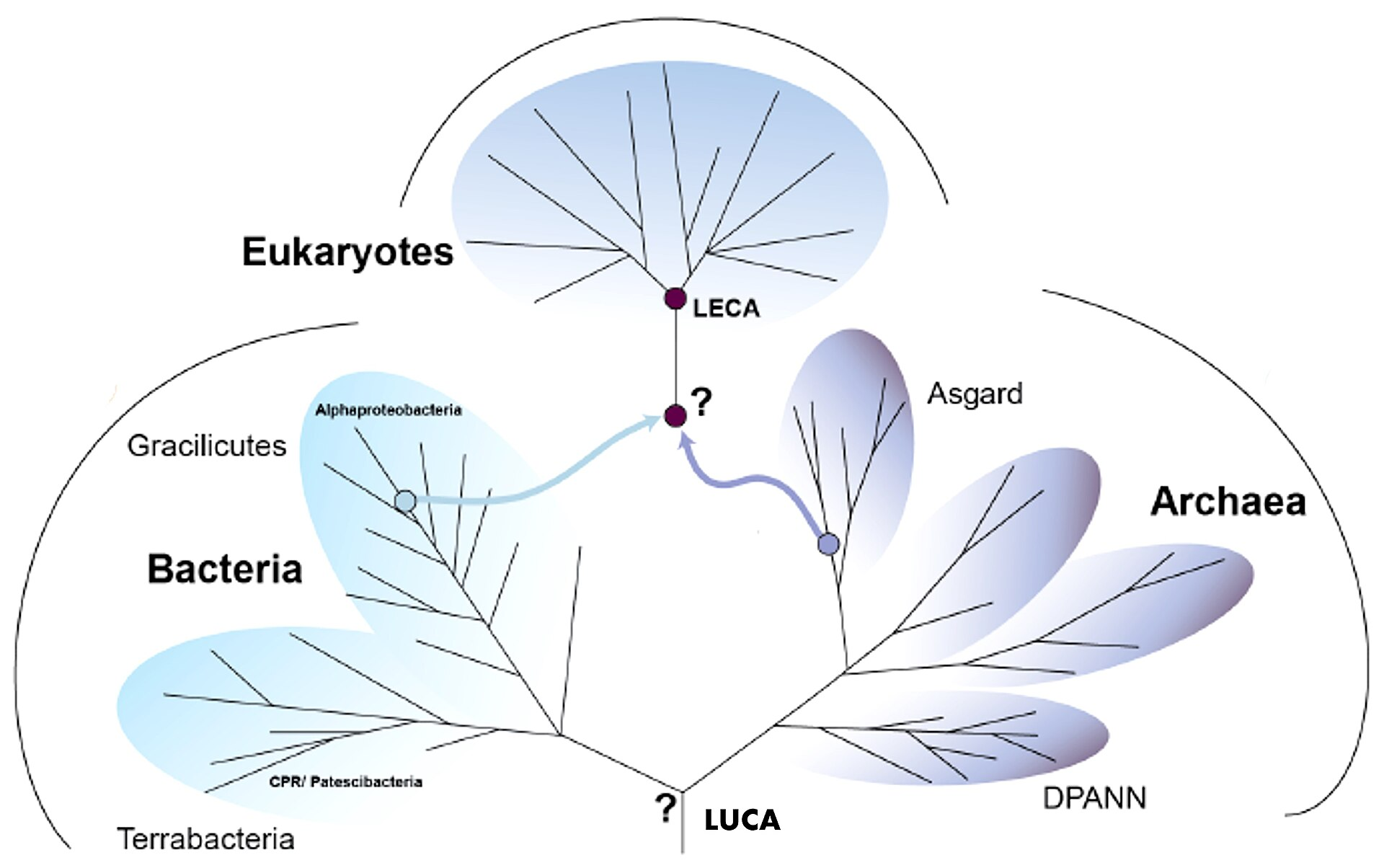
Last time, we reconstructed the nature of LUCA, the root at the tree of life. Today, we’re going to be taking a deeper look at how life makes a living: how cells harvests electricity to build more of themselves.

Life requires energy influx. Energy influx creates disequilibria and maintains them against relaxation. Some disequilibria are differences between locations. A temperature gradient, a pressure difference, and a concentration difference across a membrane are spatial disequilibria, and they relax by transport. Other disequilibria are differences between the present state of a system and an equilibrium state it can reach without moving anywhere. A supersaturated solution, a mixture of hydrogen and oxygen, and an activated molecule such as ATP or a thioester each hold a state disequilibrium, and they relax by transformation.

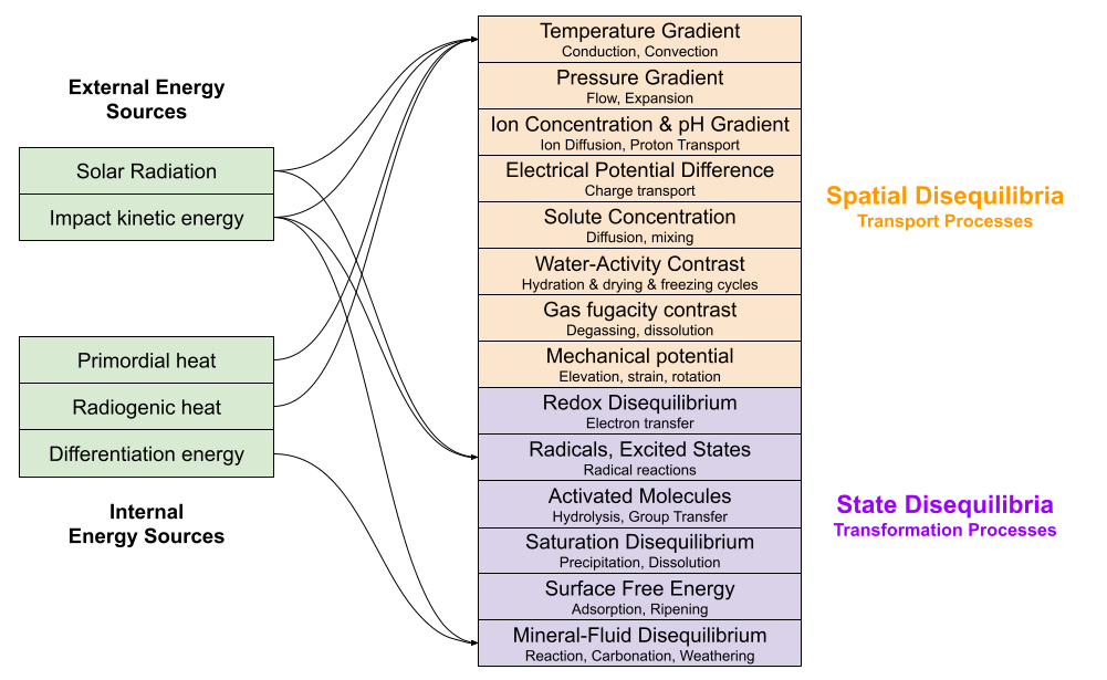
Out of this menu of fourteen options, life runs a state disequilibrium called redox.  Oxidation is electron loss, reduction is electron gain (recall the mnemonic OIL RIG). Redox (reduction-oxidation) reactions involve both of these as electron transfer dissipates this disequilibrium. 

The remainder of this post will explore how life uses redox, and where these disequilibria come from.

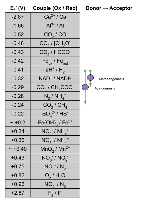
A redox couple is the oxidized and reduced form of the same chemical species. When hydrogen gas (H₂) is oxidized, its bond breaks and it releases two electrons, becoming 2H⁺. When carbon dioxide (CO₂) accepts eight electrons (along with eight protons), it is ultimately reduced to methane (CH₄) and water. A donor-acceptor pairing combines two such half-reactions. We write this pairing as 2H⁺/H₂ → CO₂/CH₄. 

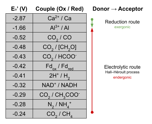
Each couple has a characteristic voltage known as the reduction potential (Eo’). Strongly negative values indicate a couple that gives electrons up readily; positive values represent willingness to accept. Spontaneous donor-acceptor pairings run from smaller reduction potentials to larger. The potential difference ΔE°′ = E°′(acceptor) − E°′(donor) must be positive. Since 2H⁺/H₂ sits at −0.41 V, and CO₂/CH₄ is −0.24 V (potentials at pH 7 from Thauer et al 1977), a methanogen running from hydrogen gas to carbon dioxide gets ΔE°′ = (-0.24) – (-0.41) = 0.17 V. Actual potentials shift with concentrations, gas pressures, and pH, so the available energy depends on the organism’s conditions. 

These relationships are often represented with a redox tower. This is done by sorting couples by reduction potential, and inverting the y-axis. The low reduction potentials (strong donors) sit at the top, and the high values (strong acceptors) are at the bottom. Spontaneous donor-acceptor pairings with positive potential difference can be represented as arrows cascading down the tower. Importantly, the magnitude of the potential difference (arrow length) determines the energy released: ΔG°′ = −nFΔE°′, where n is the number of electrons transferred and F is Faraday’s constant.

Electrochemical Cells

Redox disequilibria relax by transformation: electrons transfer in situ. An electrochemical cell separates the two half-reactions in space, connecting a state disequilibrium (the redox gap) to a spatial one (a voltage across space). Oxidation (electron donation) takes place at the anode, reduction (acceptance) takes place at the cathode. Electrons travel from anode to cathode through a conductor. The accumulating charge differences would quickly squelch the redox reaction. To achieve a cell rather than a capacitor, an electrolyte (e.g., salt solution) carries ionic current between the reaction sites. This closes the circuit and balances charge. 

We might distinguish between two forms of cell. In a galvanic cell, the donor-acceptor pairing is spontaneous (exergonic). Galvanic cells convert chemical potential into work. They “discharge the battery.” In an electrolytic cell, the donor-acceptor pairings are non-spontaneous (endergonic). These cells consume work to generate chemical potential. They “charge the battery.” 

We will soon learn that biological cells are electrochemical cells. To better contextualize this fact, we first turn to non-biological examples. 

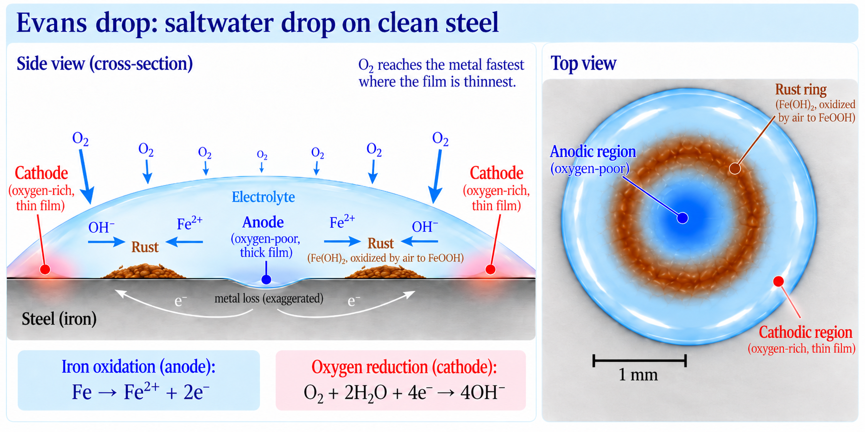
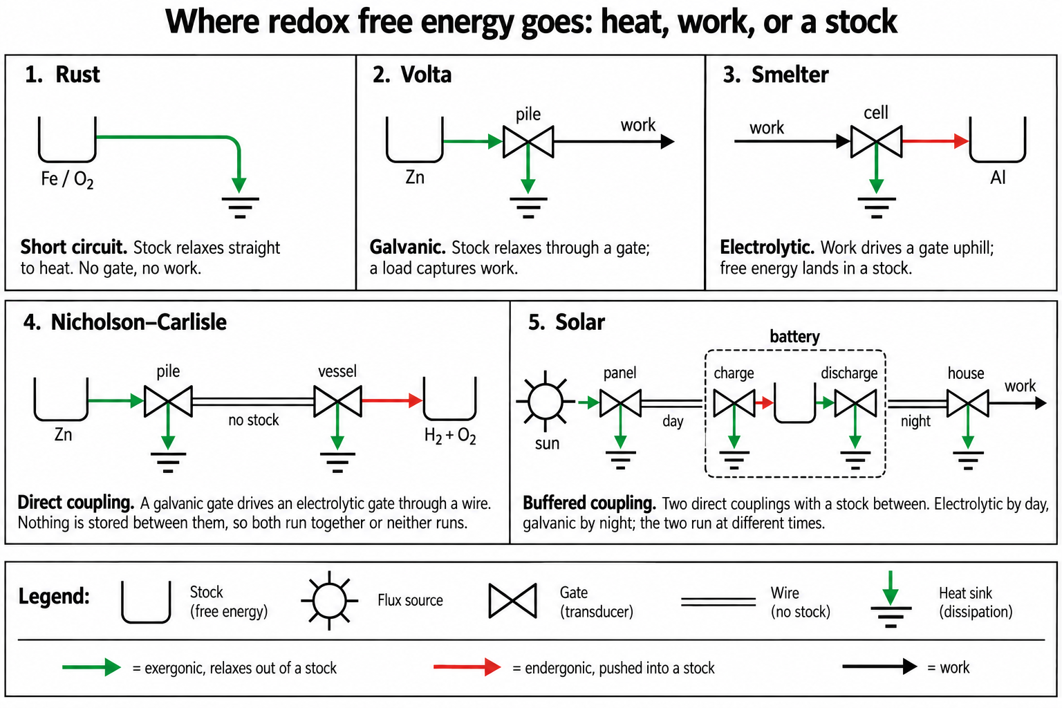
Consider the Evans experiment, a single drop of water placed on clean steel. Oxygen reaches the metal fastest near the border of the drop, where the film is thinnest, and slowest at the center. The oxygen-poor center becomes the anode, where iron is oxidized to Fe²⁺ and releases electrons. The oxygen-rich periphery becomes the cathode, where dissolved oxygen accepts those electrons and is reduced to OH⁻. Fe²⁺ and OH⁻ diffuse towards each other and precipitate, producing a characteristic ring of rust. These corrosion processes are ubiquitous because they are exergonic and, on iron, unburdened with a protective oxide film. But here, electron flow is effectively short-circuited through the metal itself. The available Gibbs free energy is dissipated mainly as heat. 

This same process can be harnessed to do work. Alessandro Volta opened the short circuit in 1800. His voltaic pile consisted of repeated zinc–electrolyte–copper sandwiches, each forming a galvanic cell.  Zinc oxidation releases electrons, which are consumed by a reduction at the copper electrode. Because the electrodes are separate pieces of metal, the electrons cannot pass directly between them. They must travel through an external wire, and anything placed in that path, which we will call the load, can capture part of the redox free-energy drop as useful work.

The pile runs because zinc oxidation is downhill. But many reactions we want run uphill. Aluminum is a prized metal, yet on Earth nearly all of it is bound to oxygen. Smelters convert aluminum oxide (Al₂O₃) into aluminum metal by adding three electrons: Al³⁺ + 3e⁻ → Al. Aluminum is a very weak oxidant, with a −1.66 volt potential. Alumina can be reduced with a stronger reductant. Deville did this in 1854 with sodium metal. But the sodium was difficult to manufacture, and aluminum production was as expensive as silver. The Hall–Héroult process lowered costs by instead supplying reducing power directly from electricity. Alumina is dissolved in molten cryolite, and a large current drives the reduction of Al(III) at the cathode to liquid aluminum while carbon is oxidized at the anode. This reaction is non-spontaneous without an external power source. This is why the industry calls aluminum congealed electricity. The metal is a stock: a reservoir of free energy, filled by one process and drained later by another. 

What provides work to an electrolytic cell? A galvanic cell can. Within weeks of Volta’s discovery, Nicholson and Carlisle placed the pile’s wires in water and watched hydrogen and oxygen appear. The voltaic pile supplied the 1.23 volts needed to decompose water. The wire connects driving and driven processes. This wire cannot sustain the reaction when the battery depletes. Both processes must proceed in tandem. In direct coupling, a driving process and a driven process are joined without enough storage to separate their operation in time. 

Direct coupling is insufficient when energy inflow and outflow proceed at different times and different rates. Consider an off-grid solar installation. During the day the panels supply electrical work, but a house draws power continuously. This setup is enabled if a stock is placed on the wire. By day, the stock (a battery) is charged in an electrolytic process. But whenever the house needs power, the battery discharges in a galvanic process. In buffered coupling, a stock separates two processes in time. The stockis filled when power is available and depleted when it is needed. A single cell can perform both electrolytic and galvanic roles. 

Respiration as a Galvanic Cell

Humans eat food and breathe oxygen. Why? Both are delivered to our cells where electrons are stripped from organic matter and sent down the respiratory chain to oxygen. Cellular respiration is a donor-acceptor pairing. Life runs on redox chemistry. 

Consider Cupriavidus necator, a bacterium that strips electrons from hydrogen to give to oxygen. We’ve already seen the electrolytic cell from the Nicholson-Carlisle experiment, which consumed energy to separate water. In 1839, William Grove constructed the reverse. He placed platinum electrodes in separate tubes of hydrogen and oxygen, connected them through an acid, and observed a current. Cupriavidus harvests energy in precisely the same way as Grove’s device: 2H⁺/H₂ against O₂/H₂O. But life utilizes this energy differently, as we will see below. 

Respiration occurs in the electron transport chain (ETC). While the modern ETC has many components, for our purposes we consider three. Electrons are passed from the entry enzyme towards the exit enzyme, which function as anode and cathode respectively. 

The entry enzyme and the exit enzyme differ across organisms. The quinone pool represents their interface. The entry enzyme (e.g., a membrane-bound hydrogenase) must accept electrons from a redox donor and reduce quinone. Quinone takes the two electrons and, from the inner face, two protons, becoming quinol. The exit enzyme (e.g., quinol oxidase), needs only oxidize quinol. (In mitochondria an extra stage, Complex III and cytochrome c, sits between the pool and the exit enzyme.)

The journey of electrons occurs without a wire. Within the proteins, an electron will tunnel between fixed metal centers, iron-sulfur clusters and hemes, spaced no more than about 14 Å apart (Page et al 1999). Between proteins, the electrons continue their journey hitching a ride on the quinone. 

Where does the work go? The ETC enzymes are all embedded in a lipid membrane, which in prokaryotes separates the cytoplasm inside from the periplasm outside. The entry enzyme oxidizes the donor and releases its protons in the periplasm. Quinone is reduced in the membrane and takes its two protons from the cytoplasm. The exit enzyme oxidizes quinol and releases those protons on the periplasm, and reduces the acceptor with further protons drawn from inside. Every pair of electrons that journeys from anode to cathode carries several protons from inside to outside. Redox is a driving process; the protein gradient is a driven process. This coupling of state to spatial disequilibrium is called chemiosmosis. 

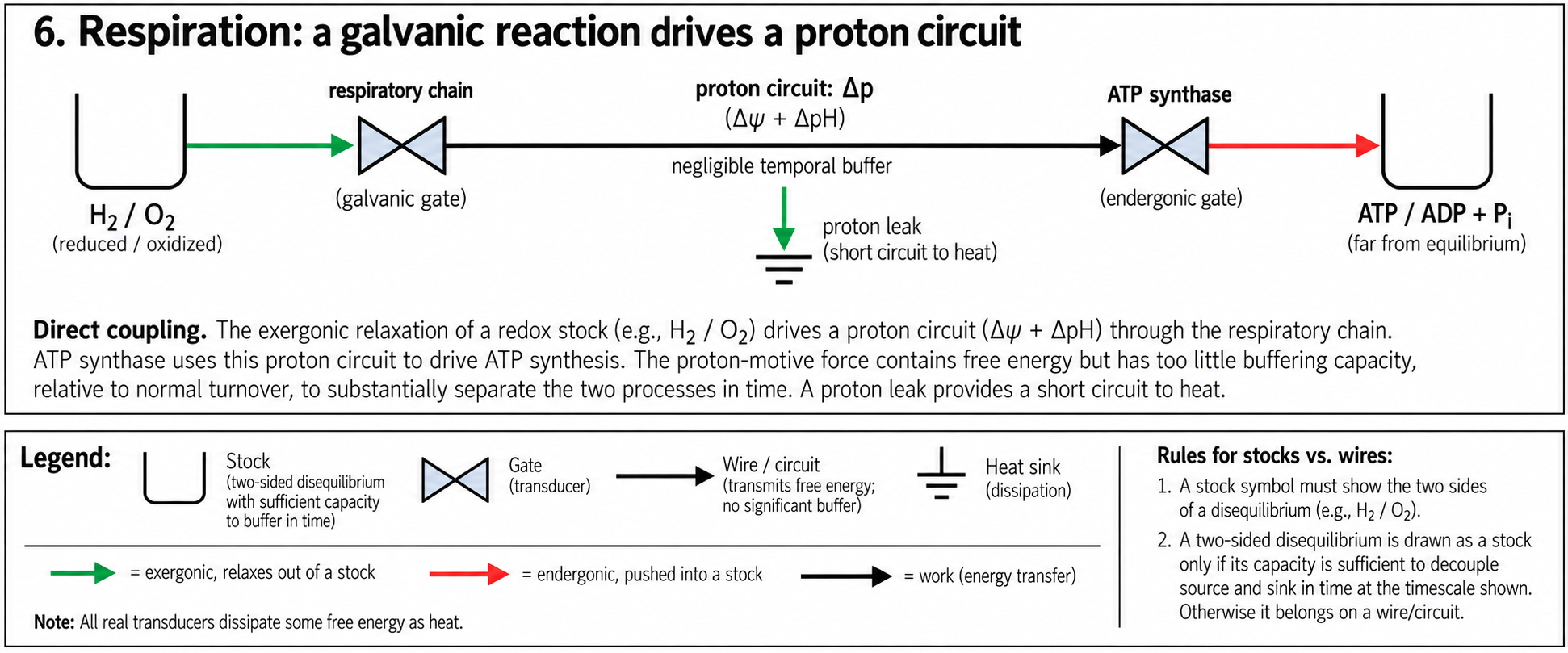
The gradient has an electrical part, Δψ, and a chemical part, ΔpH, and Mitchell (1961) combined them into a single quantity, the proton-motive force (PMF): Δp = Δψ − 59 mV × ΔpH at 25 °C. In mitochondria and most bacteria Δp is 150 to 220 mV, most of it electrical. That is roughly 15 to 20 kJ per mole of protons, and across a membrane 5 nm thick it is a field of about 4 × 10⁷ V/m, ten times the field at which air breaks down and lightning strikes (Lane 2005). Yet despite its strength, the PMF has limited storage capacity. If proton pumping stops while ATP synthesis continues, the gradient runs down. The PMF therefore serves mainly as the immediate link between driving and driven processes. This is direct coupling. 

ETC behavior resembles a voltaic pile. If you connect it to a load (the ATP synthase, which we will meet next), the PMF produces work. But what happens if you remove or disable the ATP synthase? In this open circuit, respiration slows because protons cannot return and Δp rises until the chain stalls against it. Chance and Williams (1955) starved the ATP synthase by withholding ADP. Respiration slowed to a crawl, only recovering when ADP was reintroduced. If the membrane develops a leak, this powerful voltage would be discharged in a short circuit. This is how brown fat warms newborns through a regulated leak channel, UCP1. An uncontrolled leak is more dangerous, thermodynamically equivalent to burning sugar via combustion. A short circuit releases the disequilibrium into waste heat, without powering the ATP-producing load.

The PMF produced by the ETC is only biologically useful if it performs work. That work happens at the ATP synthase. This rotor produces an activated molecule known as adenosine triphosphate (ATP). Thermodynamics favors hydrolysis of its terminal phosphate bond, leading to more stable adenosine diphosphate (ADP). Proton flux turns the synthase rotor, and the rotation forces ADP and phosphate together on the inner face. Three to five protons pass per ATP, depending on the organism. This process holds ATP, relative to ADP and phosphate, some ten orders of magnitude above the level equilibrium would allow. 

The ATP stock provides a buffer, but it is small. A human turns their whole ATP stock over within a minute or two, working muscle within seconds. The body regenerates roughly its own mass in ATP each day. ATP is called the energy currency of the cell. In many metabolic processes, ATP is used to enable non-spontaneous reactions by the group transfer mechanism. The terminal phosphate is handed to a substrate, which is lifted into a less stable state, and the endergonic step that follows is paid for by the relaxation of ATP toward ADP. Most endergonic steps in metabolism are paid this way. The rest are paid in reducing power, as we will see shortly.

Biological supply and demand rarely coincide. A plant captures sunlight by day but respires continuously. An animal eats at intervals and works continuously. A bacterium meets its substrate in pulses. Our solar-powered house solved this mismatch with the battery. Cells achieve the same buffered coupling solution with hierarchical storage. Phosphate reserves can become ATP directly. But a cell can dissolve only so much. Any reserve held in solution, like phosphocreatine in muscle, is shallow. Carbon-fuel reserves bypass this constraint by leaving the solution via polymerization (which cuts the particle count dramatically) or phase separation. Carbon-fuel reserves (including glycogen, starch, fat, and PHB) thereby unlock much deeper capacity and can last from hours to months. They rely on metabolic processes to convert their redox disequilibrium back into ATP.

We have sketched how redox disequilibrium is harvested to produce the PMF and ATP. But which molecular species does life harvest? 

Modularity and Habitat Colonization

The remarkable fact is that life does not care which span. Animals transfer electrons from organic carbon to oxygen. Prokaryotes can instead use donors and acceptors drawn from minerals, dissolved compounds, and gases. The same ETC (quinone pools, iron-sulfur clusters, a rotary ATP synthase) serves an astonishing diversity of habitats. The entry and exit enzymes are simply swapped. Life most likely began with a single donor-acceptor coupling. But modern life uses modular respiration. Donor and acceptor are configurable; the electron transport chain is largely conserved (Jelen et al 2016).

The voltage gap between an organism’s electron donor and acceptor sets the energy it can extract per electron. Power also requires current: a supply of donor and acceptor in the same place. Because life runs in water, the voltage gap has a ceiling. A substance strong enough to change the oxidation state of water will react with the solvent and cannot reach the organism. “Hydrogen gas (E°′ = −0.41 V) is the strongest reductant that accumulates in water, and O₂ (E°′ = +0.82 V) is the strongest oxidant that is both abundant and stable in it. As a stylized fact, the largest redox gap available in water is about 1.2 volts.

But on the Hadean Earth, oxygen was absent in bulk because nothing besides water photolysis produced it. The first bioenergetic revolution was the origin of life itself. The best electron acceptors available (carbon dioxide, -0.24 V; ferric iron, ≈ 0.0 V) sat within 0.5 volts of organic carbon. Limited by donor supply, the anaerobic biosphere could fix ~10¹³ mol C per year, or ~0.1 TW (Crockford et al 2023). 

Oxygenic photosynthesis heralded the second bioenergetic revolution. Cyanobacteria pushed electrons from water (+0.82 V) into carbon (-0.43 V). Water is inexhaustible, so primary production rose by an order of magnitude, to ~10¹⁴ mol C per year or ~1 TW. The waste product oxygen eventually accumulated in the atmosphere. Heterotrophs were then able to respire this span in the reverse direction. This second revolution allowed life to harvest near its maximum redox span. Subsequent revolutions had to come from current, by relaxing supply constraints.

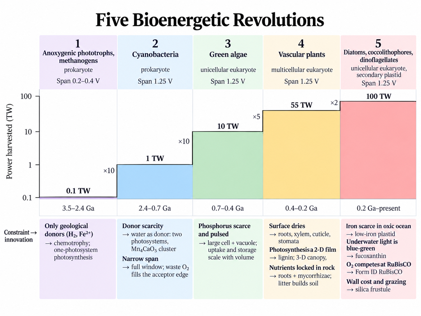
But life invaded myriad habitats in the early Earth even before oxygenic photosynthesis. The modularity of respiration allows for life to harvest nearly any form of redox disequilibrium anywhere.

A pair of electrons falling 1.23 V from H₂ to O₂ pays 237 kJ per mole of H₂, while the same pair falling 0.17 V from H₂ to CO₂, the methanogen’s living, pays 33 kJ. Between them lie the denitrifiers, iron reducers, and sulfate reducers. Redox pairings correlate with sediment depth. Oxygen is consumed at the surface, followed by nitrate, manganese, iron, sulfate, then finally CO₂ at the deepest layers (Froelich et al 1979). The biosphere fully occupies the redox tower (Falkowski et al 2008).

Microbiologists have even used gaps in the tower to predict the existence of new organisms. In 1977 Engelbert Broda listed a pairing the tower permitted but no known organism used: ammonium as donor against nitrite as acceptor. He argued that such lithotrophs should exist. They were found in the 1990s (Broda 1977; Strous et al. 1999). 

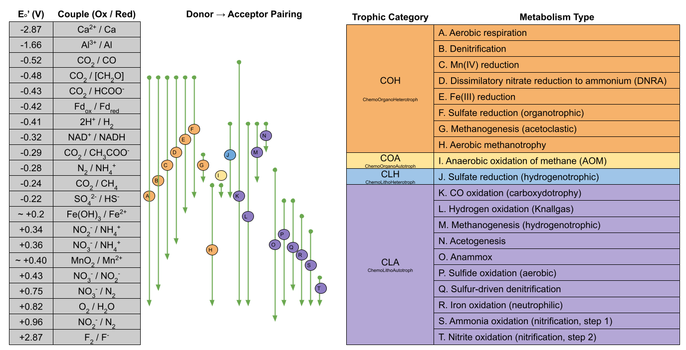
In sum, the biosphere runs galvanic cells to convert redox disequilibria into a stock of ATP. This is energy metabolism. What does a cell buy with it? 

The Machinery for Biosynthesis 

Life uses this energy to self-replicate, and making more cells requires synthesizing biomass. Energy metabolism finances carbon metabolism.

Let’s review how redox chemistry interacts with organic chemistry.  Autotrophs consume CO₂ and convert it into organic matter via carbon fixation. Carbon fixation transfers two electrons at a time from reductants to carbon. Each transfer moves a carbon atom one rung along a ladder. Define L as the total bond order from a carbon to oxygen, nitrogen, or sulfur, with a double bond counting twice.  As L decreases, the atom transforms from CO2 to carboxyl to carbonyl to alcohol to hydrocarbon. 

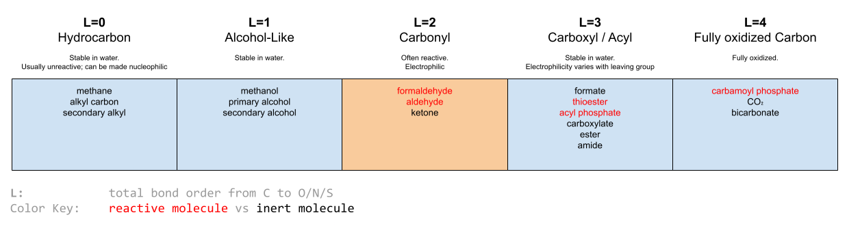
Losing L means reducing carbon. But redox does not uniquely constrain carbon chemistry. For bond formation, what matters is the local distribution of those electrons. An electrophile is an electron-poor atom that accepts electrons to form a bond, while a nucleophile is an electron-rich atom or group that donates it. Carbonyls expose a C=O bond, which is electrophilic. Hydrocarbons and alcohols do not expose this, while carboxylates at L = 3 stabilize theirs through resonance and negative charge. 

Biomass is deposited as alcohols and carboxyls, and depleted in carbonyls (Jinich et al 2020).  Yet despite avoiding carbonyls, biosynthesis requires their reactivity. Most biosynthesis reactions involve a nucleophilic carbon attacking an (electrophilic) carbonyl.  This is the carbonyl paradox. 

L tracks the two-electron transfers from reductants. But the formal oxidation state (z) also tracks changes in the carbon skeleton. At a fixed L, every C-C coupling increments z and every C-C cleavage decrements it. Defining the total C-C bond order (n), one arrives at the helpful formula z = 2L – 4 + n. Formal oxidation state ranges from +4 in CO₂ to −4 in methane, and every electron added lowers it

These are carbon-level metrics. To describe a molecule, we can average the oxidation state of its constituents. Zc denotes the average formal oxidation state of a carbon molecule. Biomass sits in the middle. Bains & Seager (2012) scored ~4300 metabolites across a variety of organisms and found a narrow intermediate band, with the vast bulk of metabolites living near Zc = 0.0. Not every intermediate carbon is a metabolite. But biological intermediates are preferentially stable, with lower Gibbs energy (Jinich et al 2020). 

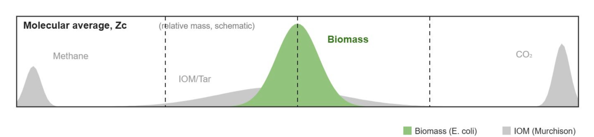
Biomass is deposited as L = 1 or 3. Biomass polarization explains how this is reconciled with Zc = 0. Fatty acids, amino acids, and anabolic carboxylates all have a reduced body around 0 and an oxidized tip at L = 3, with almost no carbon at L = 2. Sugars are the exception.

Why does life build intermediate carbon? It has tremendous combinatorial depth. Bains & Seager (2012) showed that, out of 1.7 million small molecules built from CHNOPS atoms, 95% were at intermediate oxidation state. This matters because useful biochemicals must satisfy many constraints at once. The solution space is sparse. Combinatorial depth makes selection possible. 

Intermediate carbon is also stable enough to persist in water. Water is gentle enough that most of carbon’s middle can persist. C–C, C–H, and many C–O bonds can survive long enough for complex molecules to accumulate and undergo selection (Pace 2001). Biomass polarization also helps. At cellular pH a carboxylate carries a negative charge, which keeps it dissolved in water and unable to leak through a membrane. Finally, Jinich et al. (2020) find metabolites more soluble than the nonbiological compounds of the same size that life skips.

Before carbon dioxide can be reduced, it must be activated. Activation has two components:

1. Kinetic lability lowers the barrier to reaction. Lower barriers often dramatically speed up the rate of reaction.
2. Thermodynamic driving makes a reaction energetically favorable.

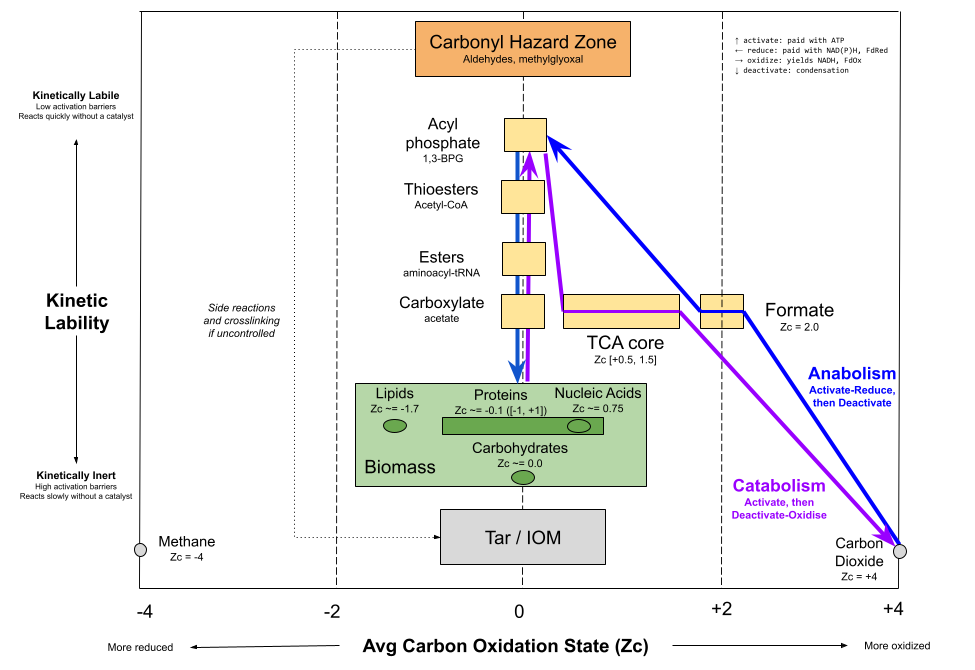
Lability and driving are often correlated, but not always. Kinetic trapping describes a metastable molecule. These products “want” to react thermodynamically, but the activation barrier precludes the reaction at reasonable time frames. Nearly all biomass is kinetically trapped. For example, ATP hydrolysis is strongly favorable, yet it persists in water because the uncatalyzed reaction is slow. Biomass remains loaded, and can be harvested for energy once an enzyme opens the barrier.  

Driving does not require a change in oxidation state. A carboxylate is stable, but replacing its oxygen with a better leaving group produces an activated acyl compound such as a thioester or acyl phosphate. The carbon stays at L = 3 throughout.

In metabolism, intermediate carbon passes through the carbonyl hazard zone. It is quickly deactivated in a chemically selective manner. Without that control, abiotic carbon can go awry. In an aldol reaction, two carbonyls enter and one exits, so the reaction can continue indefinitely.  The chemistry fans outward. Dehydration gradually pulls the survivors into aromatic rings. The resultant products include tar or insoluble organic matter (IOM). Tar is a dead end. It can burn, but no biological reaction can return it to a set of small molecules. 

To convert carbon dioxide to biomass, or vice versa, carbon must first become labile. Anabolism requires three ingredients: a carbon source, an energy currency to activate it, and a reductant currency to attach electrons to it. Consider the Calvin cycle. NADPH is too weak a reductant for a carboxylate, so ATP first converts the carboxylation product, 3-phosphoglycerate, into 1,3-bisphosphoglycerate, which NADPH can reduce. Activation comes first; reduction follows; and the product, glyceraldehyde 3-phosphate, is an aldehyde inside the hazard zone. From there the carbon descends by condensation into the forms we know as biomass.

Catabolism does not simply oxidize biomass either. It must first activate the carbon, by phosphorylation or by attachment to coenzyme A, before the oxidations run. The descent returns far more ATP than the climb cost, and the electrons removed reload the reductant pool. Anabolism and catabolism trace the same loop in opposite directions.

Reductant Carriers

We are ready to return to electrochemistry. Galvanic cells convert redox disequilibria into a stock of ATP. Cells use this energy to fix carbon. 

The requirement to reduce carbon is in tension with the modularity of respiration. What if the respiratory substrate is not strong enough to reduce carbon?  H₂S sits at −0.27 V, NH₄⁺ at +0.34 V, NO₂⁻ at +0.43 V, and Fe²⁺ at +0.77 V in the acidic water where the best-studied iron oxidizers grow. All of these are far weaker donors than biosynthesis requires. How do these cells reduce carbon uphill?

To address this, life routes biosynthetic electrons through two universal reductant carriers. The nicotinamide cofactors NAD(P)H sit at −0.32 V under standard conditions. Ferredoxin, a small iron-sulfur protein, sits between −0.40 and −0.50 V depending on the organism. Once carbon is activated, NAD(P)H can reduce it, and it serves nearly all biosynthetic reductions. Ferredoxin covers the few steps that need a stronger reductant. After donating electrons to biosynthesis, these carriers return in their oxidized forms and must be reduced again.

A reduction carrier provides other benefits beyond enabling the reduction of carbon. The diversity of respiration enables flexible energy capture. But it would be inefficient to tune thousands of metabolic pathways to many dozens of environmental reductants. The reduction currency provides modularity: an adaptor layer between energy capture and biosynthesis. It also provides regulation. Rather than leaving reductants at the potential and concentration imposed by the local habitat, the cell can maintain its reductant pools at controlled redox states. For example, NAD(P)H potential is ideally suited to keep dangerous carbonyls at low steady-state concentration (Jinich et al 2018).

But how does a cell finance carrier recycling? When the environmental reductant is lower potential than the reductant carriers, carrier recycling doesn’t require energy. Hydrogen-eating autotrophs can produce NADH directly, because hydrogen at nominal conditions sits above NAD on the tower. Heterotrophs can reduce their carriers for free as well. The electrons in organic carbon span a wide range of potentials, and metabolism harvests only the deepest ones. 

But what happens when the environmental reductant is weaker than the carrier? In that situation, carrier recycling requires work. This is where life can manifest its metabolism as an electrolytic cell. 

The Electrolytic Cell

We met electrolytic cells in industrial reduction of alumina to aluminum. If stronger reductants are unavailable, the smelter can deploy external work, and leave that work embodied in the metal. If no stronger reductants are available to life, it can harness PMF from its galvanic cell to perform carrier recycling. Then biosynthesis drives CO₂ to biomass from the reductant carriers. Biomass is congealed electricity. 

When reductant recycling is not free, biology has found two ways to fund it with redox disequilibria.

First, reverse electron transport (RET) can pay from the wire. The PMF can push electrons from the quinone pool to NAD⁺, or from H₂ to ferredoxin. Complex I does this in nitrite and iron oxidizers. Ech does this in methanogens that carry cytochromes.

Second, electron bifurcation also taps energy metabolism, but pays earlier. Bifurcation takes an electron pair from a weak reductant and splits it: one electron falls to a high-potential acceptor, and the energy released pays for lifting the other onto ferredoxin.

Both of these solutions involve a redox disequilibrium powering two loads in parallel: synthesizing energy currency and reductant carriers. Energy metabolism and carbon metabolism compete. But there is another way to synthesize reductants without drawing on a redox disequilibrium. 

Light can serve the same purpose. A photosynthetic reaction center absorbs a photon and returns the electron at a lower potential than it received. The photon raises the electron by more than one volt, but part of that energy is spent to make the reaction irreversible. The resultant voltage gain (about 0.5 volts) subsidizes carrier recycling.  A chemotroph needs an environmental reductant above its carriers on the tower, or it pays for the lift with bifurcation or RET. But an anoxygenic phototroph can use an environmental reductant that is 0.5 volts weaker, because light pays for that part of the lift. 

Two families of reaction centers exist. 

Purple bacteria carry the type II reaction center, which deposits its electron in the quinone pool. The electron travels through the ETC cyclically, and produces PMF. Quinol is a weaker reductant than NADH, so reductant recycling must use RET. The purple bacterium converts PMF into reductant.

Green sulfur bacteria carry the type I reaction center, which deposits its electron in ferredoxin. Light pays for reductant recycling directly. Electrons reach the reaction center through the ETC, making PMF along the way. They come from the environmental reductant, or from ferredoxin sent back around the loop. The green sulfur bacterium spends reductant to make PMF, the reverse of the purple bacterium. 

Light arrives by day, but energy expenditure is continuous. Every phototroph relies on carbon-based storage to bridge the gap. Bacteria use glycogen; plants use starch. The stock is filled by electrolytic anabolism by day, and drained by galvanic catabolism by night. The structure mirrors the solar-power battery bank: two direct couplings separated in time by a stock. 

Oxygenic photosynthesis wired both reaction centers in series. The type II center moves electrons from water to the quinone pool. Their descent through the ETC produces energy. The type I center lifts the electrons into a ferredoxin carrier. These photons together pay the whole 1.25 volt span. This was the second bioenergetic revolution.

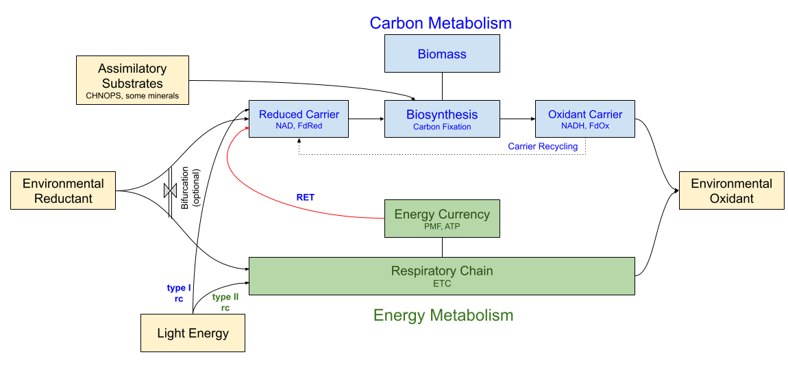
To sum up, galvanic and electrolytic circuits can coexist. The galvanic circuit harvests the environmental redox gradient as PMF. The electrolytic circuit uses PMF to lift electrons onto the carriers, to enable biosynthesis. A nitrite oxidizer runs both circuits continuously. A phototroph decouples galvanic and electrolytic circuits, with carbon-based storage as the “battery” stock in between.

One question remains. If life harvests redox gradients, what creates the gradients in the first place? 

A Planet-Sized Battery

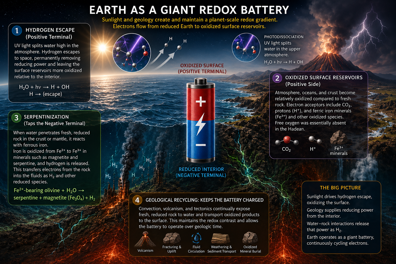
The battery existed before life learned to tap it. The Earth is a planet-sized redox battery (Smith & Morowitz 2016). Its anode is the mantle, rich in ferrous iron. Its cathode is the ocean and atmosphere, rich in carbon dioxide. The resultant redox span from H₂ to CO₂ is 0.2 volts. LUCA tapped this battery first. Plug-and-play respiration came later.

The atmosphere was birthed from volcanic degassing. This process built an oxidizing atmosphere of H₂O, CO₂, N₂, and SO₂. Photodissociation further oxidized the planetary cathode. Ultraviolet light breaks down water in the stratosphere. Hydrogen is prone to escape into the exosphere. The remaining oxygen is electron-hungry, oxidizing whatever it meets. Escaping hydrogen oxidizes our surface (Catling et al 2001). On Earth the process is slow, because the tropopause cold trap freezes water out before it reaches the stratosphere (Catling & Kasting 2017). Venus had no such trap, and photodissociation cost it an ocean (Kasting & Pollack 1983).

The mantle is rich with ultramafic rock, with a great deal of ferrous iron in olivine and pyroxene. Ferrous iron (Fe²⁺) holds one electron more than ferric iron (Fe³⁺), and loves to shed electrons. Serpentinization occurs when seawater reaches this rock. Ferrous iron gives its electron to water, ferric iron is left behind in magnetite and serpentine, and the electron leaves as H₂. H₂ carries the mantle’s reducing power, bringing the planetary anode up into the ocean. 

The two terminals do not discharge spontaneously. 4H₂ + CO₂ → CH₄ + 2H₂O is kinetically trapped. The reaction needs a catalyst. Life bridges the gap.

Other planets have iron and water, and some have freed oxygen by photodissociation. But corrosion usually stops. As the surface rusts, the electron-rich iron below becomes blocked. Current persists where fresh rock continues to meet water. On Earth, plate tectonics exposes fresh ultramafic rock at ridges, and subducts oxidized crust. But tectonics is not a hard requirement. Enceladus produces redox disequilibria from a porous core repeatedly damaged from tidal forces (Waite et al. 2017). 

Modern serpentinization yields ~10¹² mol of H₂ per year (Cannat et al. 2010; Worman et al. 2016). At 0.2 volts that is ~1.2 GW of chemical power. This planetary battery may have generated enough power to spark the first bioenergetic revolution (Russell et al. 2010).

Until next time. 

References

• Bains & Seager (2012). A combinatorial approach to biochemical space: description and application to the redox distribution of metabolism.
• Broda (1977). Two kinds of lithotrophs missing in nature.
• Cannat et al (2010). Serpentinization and associated hydrogen and methane fluxes at slow spreading ridges.
• Catling & Kasting (2017). Atmospheric Evolution on Inhabited and Lifeless Worlds.
• Catling et al (2001). Biogenic methane, hydrogen escape, and the irreversible oxidation of early Earth.
• Chance & Williams (1955). Respiratory enzymes in oxidative phosphorylation. III. The steady state.
• Crockford et al (2023). The geologic history of primary productivity.
• Falkowski et al (2008). The microbial engines that drive Earth’s biogeochemical cycles.
• Froelich et al (1979). Early oxidation of organic matter in pelagic sediments of the eastern equatorial Atlantic: suboxic diagenesis.
• Jelen et al (2016). The role of microbial electron transfer in the coevolution of the biosphere and geosphere.
• Jinich et al (2018). Quantum chemistry reveals thermodynamic principles of redox biochemistry.
• Jinich et al (2020). A thermodynamic atlas of carbon redox chemical space.
• Kasting & Pollack (1983). Loss of water from Venus. I. Hydrodynamic escape of hydrogen.
• Korenaga (2013). Initiation and evolution of plate tectonics on Earth: theories and observations.
• Lane (2005). Power, Sex, Suicide: Mitochondria and the Meaning of Life.
• Mitchell (1961). Coupling of phosphorylation to electron and hydrogen transfer by a chemi-osmotic type of mechanism.
• Pace (2001). The universal nature of biochemistry.
• Page et al (1999). Natural engineering principles of electron tunnelling in biological oxidation–reduction.
• Russell & Hall (1997). The emergence of life from iron monosulphide bubbles at a submarine hydrothermal redox and pH front.
• Russell et al (2010). Serpentinization as a source of energy at the origin of life.
• Sleep et al (2004). H₂-rich fluids from serpentinization: geochemical and biotic implications.
• Smith & Morowitz (2016). The Origin and Nature of Life on Earth: The Emergence of the Fourth Geosphere.
• Strous et al (1999). Missing lithotroph identified as new planctomycete.
• Thauer et al (1977). Energy conservation in chemotrophic anaerobic bacteria.
• Waite et al (2017). Cassini finds molecular hydrogen in the Enceladus plume: evidence for hydrothermal processes.
• Worman et al (2016). Global rate and distribution of H₂ gas produced by serpentinization within oceanic lithosphere.