Followup To: Potential Outcome Models
Part Of: Causal Inference sequence
Content Summary: 900 words, 9 min read

Recap

Our takeaways from last time:

• Questions of causality have interesting links to “what if” questions (counterfactuals)
• We can construct a Possible Outcomes model that deploys counterfactual reasoning to explain observed effects
• If we reverse the direction of a Possible Outcomes model, we see that observed reality only partially determines our counterfactual knowledge.
• If we look carefully at the relationship between observed variables and their counterfactual implications, we can begin to see a pattern.

Today, we will connect our Possible Outcomes Model back to causality. But first, we must address questions of scale!

Scaling Up Potential Outcome Models

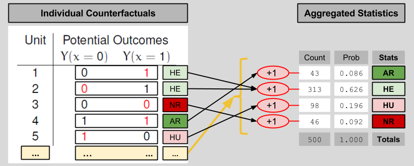
In order to get a sense for the performance of the drug as a whole, one needs to view its effects on a larger population. The above table has N=5 subjects. Let’s imagine 500 subjects instead. Fortunately, if we don’t want to deal with 500 row tables, we can aggregate the data into a shorter entry. Here’s one possible way to compress a large counterfactuals table into four entries:

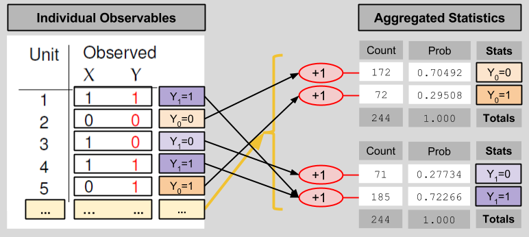
We compress the observables table in an analogous manner:

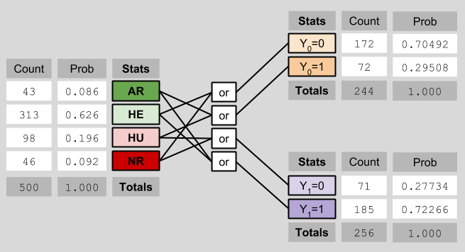
These statistical results relate to each other in the following way:

Average Causal Effect

Let us now shift our gaze from machinery to our original motivation. How might we use potential outcome models to estimate causal effect? If most of our patients are of type NR or AR (Never/Almost Recover), that would suggest that our drug is exerting negligible causal muscle over the patients. However, a drug that indexes many patients of type HE (Helped) seems to have an effect. Conversely, a drug that creates many HU (Hurt) patients can also be said to have a medical impact. Let us create one measure to index both; let Individual Causal Effect (ICE) represent:

ICE = Y₁ – Y₀

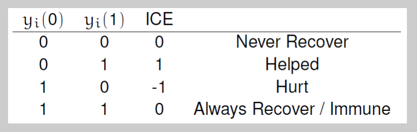
Another way of putting the above paragraph, then, is that causally-interesting patients are those with a non-zero ICE score.

As we scale up our model, our causal measure must follow suit. Let Average Causal Effect (ACE) represent:

ACE = P(HE) – P(HU)

In our case (see the diagram about ICE), the ACE = 0.626 – 0.196 = 0.43.

Learning ACE Bounds

Let’s put on our Learning Mode Glasses, and recall that we are unable to observe P(HE) nor P(HU). Instead, we can only view X and Y. What can we learn about the ACE in this context? It is tempting to say “nothing”, since we cannot uniquely determine the counts of the four outcome types. But this would be a mistake, for we can in fact establish bounds for our ACE.

The lower bound of the ACE occurs when the maximum possible number of observed outcomes are ascribed to Hurt people, and the minimum possible number of observed outcomes are ascribed to Helped people:

Thus, the lowest possible value of the ACE is 0.000 – 0.286 = -0.286.

Analogously, the upper bound of the ACE is determinable by imagining a scenario with as few Hurt people, and as many Helped people, as possible:

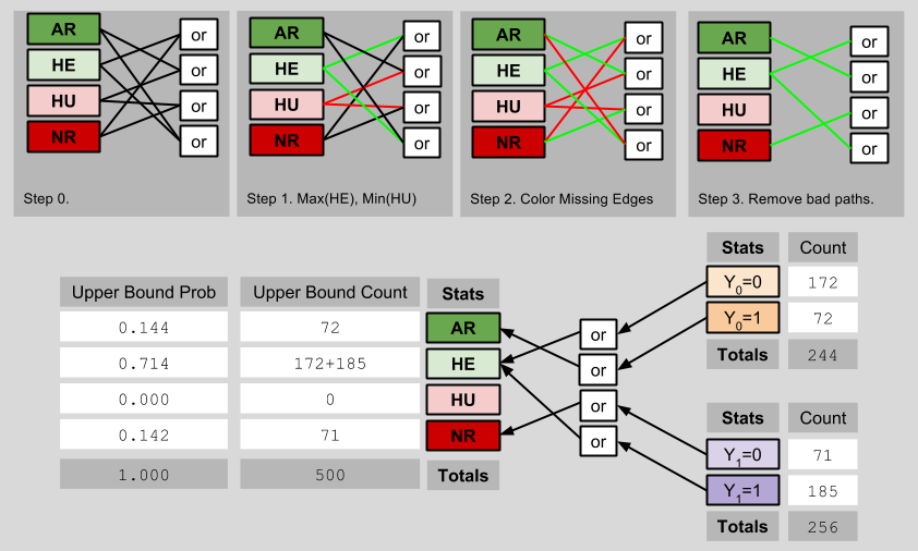
The highest possible value of the ACE is therefore 0.714 – 0.000 = 0.714. Thus, we can see that (despite not knowing the true ACE), we have shrunk its possible values from [-1, 1] to [-0.286, 0.714]. Importantly, this smaller fence still contains the true ACE of 0.43.

Transcending ACE Bounds

Can we do better than this? Yes. Let us recall an axiom we used to build our Potential Outcomes Framework:

Consistency Principle: Y = Y₁* X + Y₀*(1-X)

This principle is saying nothing more than that the red numbers on our potential models diagrams must match:

It turns out that, if you are willing to purchase an assumptions, you can estimate the true ACE from observed data alone.

Randomization Assumption: selection variable X is independent of the counterfactual table (X ⊥ Y₀, Y₁)

If the Randomization Assumption is true, then we may derive the following startling fact:

P(Y=i|X=1)

= P(Y₁=i|X=1) # Because of Consistency Principle

= P(Y₁=i) # Because of Randomization (X ⊥ Y₁)

= P(Y₁=i, Y₀=1) + P(Y₁=i, Y₀=0) # Marginalization over Y₀

When i=0, we have P(Y₁=0) = P(HU)+ P(NR). When i=1, we have P(Y₁=1) = P(HU)+ P(NR)

By the same logic, we can condition on X=0:

P(Y=i|X=0)

= P(Y₀=i|X=0) # Because of Consistency Principle

= P(Y₀=i) # Because of Randomization (X ⊥ Y₀)

= P(Y₀=i, Y₁=1) + P(Y₀=i, Y₁=0) # Marginalization over Y₁

When i=0, we have P(Y₀=0) = P(HE)+ P(NR). When i=1, we have P(Y₀=1) = P(AR)+ P(HU)

These four facts together exhibit startling similarities to one of our results from last time:

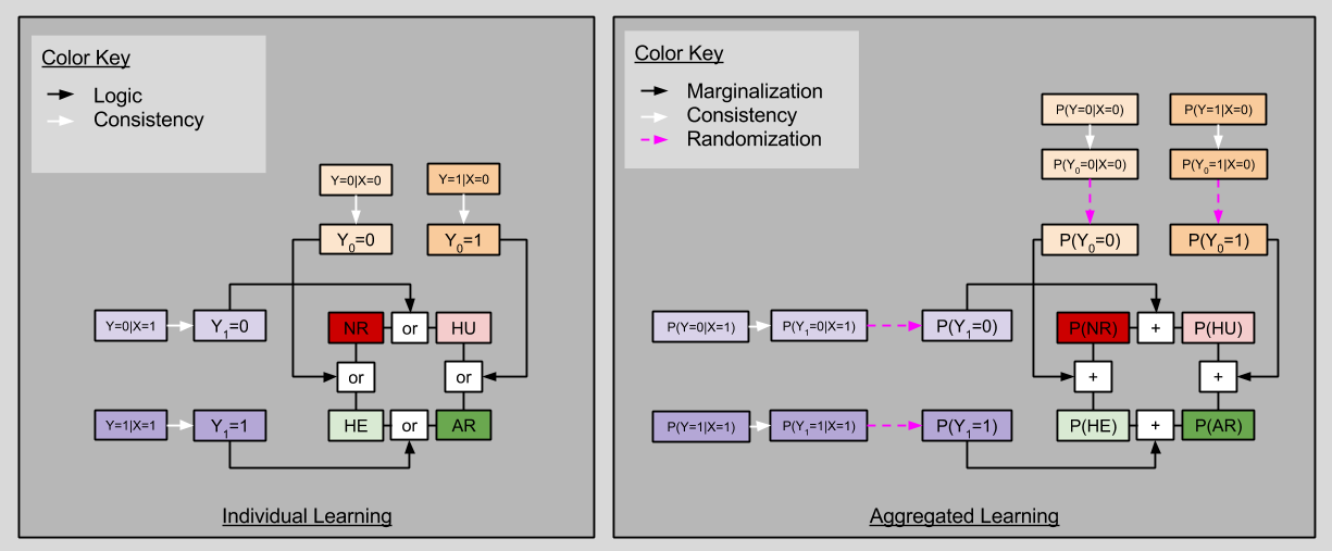
Notice that, although we can never uniquely determine say P(HU) from observables alone, we can estimate the ACE directly!

P(ACE)

= P(HE) – P(HU)

= P(HE) + P(AR) – [P(HU) + P(AR)]

= P(Y₁=1) – P(Y₀=1)

Let’s see this in action. Recall our original data, reproduced in aggregated form below:

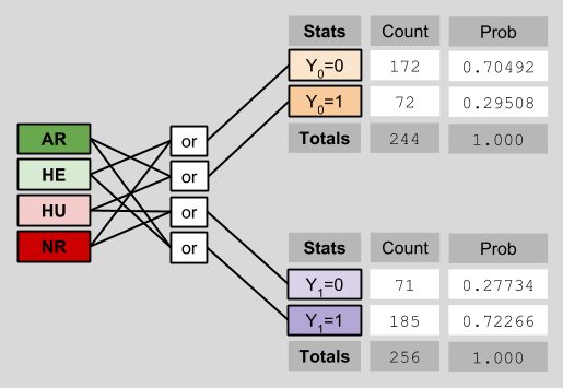
Notice that I have explicitly removed the counterfactual data previously visible on the left side of the diagram. This deletion reflects the fact that counterfactual data is intrinsically opaque to us. This depressing fact is known as the Fundamental Problem Of Causal Inference. 

Here, we can estimate the ACE as follows:

P(Y₁=1) – P(Y₀=1)

= 0.72266 – 0.29508

= 0.427528

If that’s not close to the ACE true value of 0.43, I don’t know what is. 🙂

Takeaways

• Data aggregation statistics are a useful way of summarizing large counterfactual/observable tables.
• Rubin’s potential outcome model informs philosophical questions of causality through his Average Causal Effect (ACE) measure
• In real-world scenarios, where counterfactual data is opaque to us, we can still derive upper and lower bounds for the ACE
• If we are willing to assert the independence of sampling processes, however, we are able to estimate the ACE directly!