Life’s First Ratchet

Part Of: Biology sequence
Followup To: A Portrait of LUCA
Content Summary: 4000 words, 20 min read

Cutting the Knot

Abiotic chemistry is leaky. Sugars brown into tar. Nucleic acid hydrolyzes in warm water on a timescale of days to weeks. Practically anything soluble diffuses away. Whatever complexity chemistry builds is temporary. To achieve LUCA, chemistry needed a ratchet.

The natural place to look for that ratchet is LUCA’s own subsystems, but they depend on one another. Genes prescribe proteins, yet cannot be expressed without proteins to transcribe and repair them. Metabolism supplies the materials for both, yet runs on protein catalysts that genes encode. Asking which came first is really asking which subsystem supplied the first ratchet. 

This Gordian knot is a question of functional priority. There are two ways to cut it.

One answer sees the first ratchet in nucleic acid. A system that can copy information can preserve innovation. This is the genetics-first tradition.

The other sees it in metabolism. A network that captures free energy can maintain its own organization and generate the building blocks heredity would later need. This is the metabolism-first tradition. 

The RNA World

Let’s set metabolism aside for a moment. Among the three biopolymers of the central dogma – DNA, RNA, and modern coded proteins – which came first? On this smaller question, the scientific community has achieved consensus. Metabolism-first and genetic-first camps agree: RNA came first. 

RNA is the answer because it can do both jobs. RNA stores information in its nucleotide sequence, like DNA. But it also folds itself into structures that catalyze chemical reactions, like proteins. The discovery of self-splicing introns revealed that RNA can act as a catalyst (Kruger et al. 1982). Most modern biological catalysts are protein enzymes. RNA catalysts are called ribozymes.  The universal coenzymes hint at the same history. NAD, FAD, coenzyme A, and SAM are all built on nucleotide scaffolds, which White (1976) read as molecular fossils of an RNA-based metabolism.

The ribosome is the engine of the genetic code. Remarkably, we are able to reconstruct its development at the atomic resolution. The oldest part of the ribosome, its center known as the peptidyl transferase center (PTC), contains no proteins at all. Its catalytic heart is entirely RNA. The ribosome is a ribozyme (Nissen et al. 2000). 

Other genetic polymers could, in principle, have preceded RNA. One genetic system could also have replaced another while preserving the basic function of heredity, a process sometimes called genetic takeover (Hud et al. 2013). But for now, in the name of parsimony, we will assume the first genetic ratchet was RNA. 

Why is protein-first no longer an active research tradition? Amino acids and short peptides may well predate RNA. But RNA apparently precedes modern coded proteins. The RNA World constitutes major progress in cutting the knot. The RNA world is silent on the order of metabolism. This is the residue. 

The genetics-first solution advocates a strong version of the RNA World: genetic heredity precedes the emergence of metabolism. Natural selection then improves the chemical system around the replicator. No one questions the capacity of nucleic acids to build and retain complexity. The burden is to show how geochemistry alone can birth such a wondrous digital inheritance

The metabolism-first tradition holds that metabolism existed before RNA, and therefore before genetically encoded proteins. A non-enzymatic protometabolism must exist first. This school fully accepts digital inheritance. But it proposes that protometabolism served as the first ratchet. Geochemistry is thus less burdened. The burden here is twofold: to show that non-enzymatic protometabolism is viable, and to show that a mere reaction network can preserve innovation without genes. We take up the second question in a later post.

Let us explore the viability of specific genetics-first and metabolism-first theories. These are grounded in specific habitats. But before we search for the Geography of Genesis, we must first understand what success looks like. Designing such a rubric takes us back to first principles. We begin with thermodynamics.

Life as a Dissipative Structure

Free energy is the part of energy that can do work. The second law of thermodynamics says that energy tends to spread out. Hot objects cool, gases mix, and chemical gradients become weak. 

A closed system does not exchange matter with its surroundings. Without a continuing source of usable energy, its chemical differences decay toward equilibrium. As a system approaches equilibrium, free energy is dissipated, often as heat, and less remains available to do useful work. 

Life manifests tremendous complexity and order. In What Is Life?, Erwin Schrödinger explained that life is not a closed system. An open system can exchange energy and matter, so an external process can maintain nonequilibrium conditions. Life exists in an open system.  It consumes external energy and matter, then releases heat and waste. Life keeps local order while disorder increases in its surroundings. 

The chemist Ilya Prigogine developed the idea of dissipative structures. These structures import free energy from their environment. They maintain local order by using this energy and releasing heat and waste into their surroundings. When the flow stops, the structure usually weakens or disappears. 

Dissipative structures occur at many scales. Examples include convection cells, flames, chemical oscillations, hurricanes, and living organisms. For the origin environments we will consider, two energy sources matter most: sunlight and geological activity. 

Our first requirement is sustained free-energy flux. The Garden of Eden must feature continuous (or at least recurrent) throughput sufficient to maintain far-from-equilibrium chemistry.

Chemical Selectivity

Free energy flux can drive useful reactions. It can also drive thousands of useless ones. 

In organic chemistry, a small set of reactive molecules can combine in many different ways. Each new product can then react with the original molecules or with other products. The number of possible pathways can grow rapidly. Researchers call this a combinatorial explosion

Scientific experiments (e.g., Miller Urey) and natural phenomena (e.g., carbonaceous chondrites) both tend to produce tar: complex mixtures that are difficult to separate or even characterize. 

The formose reaction gives another example. Recall that ribonucleic acid (RNA) uses one particular sugar: ribose. Under alkaline conditions, formaldehyde produces dozens of different sugars and related compounds, while ribose appears as only one component of the diverse products. As the reaction continues, useful products can disappear into still more complex chemistry. 

Life is different. Biology uses an extraordinarily restricted region of chemical space. About 500 naturally occurring amino acids have been identified, but the standard genetic code uses only 20 of these to build proteins. The same organizing principle appears in metabolism. Smith and Morowitz (2004) identify eleven TCA-cycle carboxylic acids as a universal anabolic core, from which the major pathways of biosynthesis branch. In their formulation, lipids, sugars, amino acids, nucleotides, and other major classes of biomolecules are ultimately built outward from this small conserved core. 

A biochemical environment must channel significant flux toward its target products, while limiting competing reactions. This is a second requirement for Eden: chemical selectivity

For genetics-first, this requirement must be met before selection can start. A nucleic acid is a monument of chemical selectivity: one sugar among dozens, a few bases among many, the correct linkage among several. The environment must achieve that discrimination unaided. Genetics-first chemistry therefore requires prebiotic mechanisms that narrow the product distributions. 

Metabolism-first theories propose another possibility. Positive feedback reactions (aka autocatalysis) can deliver selectivity without a special environment. But it only works if the network reinforces a restricted set of productive reactions, rather than amplifying chemical clutter. We will explore this topic in more detail in a followup post.

Deriving the Rubric

We can say more. Chemical principles allow us to derive five additional requirements. 

  1. Provenance. The required feedstocks and catalysts must arise or arrive naturally.
  2. Reactant Concentration. Feedstocks must reach concentrations high enough for useful reactions.
  3. Material Flux. Fresh material and free energy must continue to enter, while waste leaves and spent material is removed, reactivated, or recycled. 
  4. Product Retention. Useful products must also remain close by long enough to interact again, rather than immediately dispersing into the environment. 
  5. Net Production. Eden must not only produce these target products. It must produce them faster than it destroys them. We require net production.

Material flux and product retention are in creative tension. Eden must eject waste while selectively retaining useful products. 

The above concerns single reactions. But theories of abiogenesis rely on many processes.

Suppose one reaction requires acidic conditions, another alkaline conditions. Or one may require intense ultraviolet radiation, while another important product is rapidly destroyed by the same radiation. A theory may need to confine different reactions to different microenvironments. Such conflicts do not make a pathway impossible, but they do require that these microenvironments exchange products in a realistic way. This is the requirement for condition compatibility.

It is not enough to demonstrate each reaction separately in a laboratory. Products of one step must naturally reach the next without artificial purification, isolation, or reagent replacement.  This is the requirement for process continuity.

A favorable environment is of little use if it disappears before cumulative organization can develop. The environment must persist or recur often enough to provide continuity across time. Our last requirement is habitat persistence

These requirements are universal. But genetics-first and metabolism-first theories also generate idiosyncratic requirements. Let’s examine each in turn.

Building Nucleic Acid

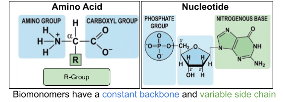
Genetics-first demands a specific product. Geochemistry must synthesize a nucleotide. Every nucleotide brings together a sugar (ribose), a nitrogenous base, and a phosphate group into a single large molecule:

Carbon, hydrogen, and oxygen are readily available in many geological habitats. Nucleotides also require nitrogen and phosphorus, and these present new challenges for genetics-first models.

Most environmental nitrogen is molecular nitrogen, N₂. The strong triple bond in N₂ makes it unusually unreactive. Before nucleotide synthesis can begin, some process must supply fixed nitrogen in a reactive form. Nitrogen fixation is one way to make it more reactive (Mateo-Marti et al. 2019). Similarly, phosphorus is present in rocks, but much of it occurs in minerals with low solubility. In water containing calcium, dissolved phosphate is quickly locked away into minerals. Many prebiotic reactions, meanwhile, require phosphate concentrations far above those found in ordinary natural waters. This is the phosphate problem (Toner and Catling 2020). Together, these problems generate two requirements. A genetics-first theory requires bioavailable nitrogen and phosphate. 

Of course, individual nucleotides aren’t enough. They must come together as long strands of nucleic acid

RNA polymerization occurs through a condensation reaction. But condensation polymerization is disfavored in water. The equilibrium instead favors the reverse reaction, hydrolysis. Joining nucleotides into a chain therefore requires an input of free energy (Yadav et al. 2020). Monomer activation denotes the requirement to store or couple this free energy so that phosphodiester-bond formation can proceed.

Providing free energy is not enough. Polymerization also requires high efficiency. A 45-nucleotide polymer requires 44 bond-forming steps. At each step, the chain can degrade. Even modest inefficiency therefore compounds across the chain. Polymer elongation denotes the requirement for bond formation to be efficient enough to produce functional-length polymers.

Towards a Replicator

We’ve established a long RNA polymer. Next, it must copy itself. 

Natural selection cannot act on sequence information until polymers are long enough for different sequences to produce different functional structures. Very short oligomers have limited capacity to fold into complex three-dimensional forms.

We do not know a strict minimum length for a useful hereditary polymer. But Gianni et al. (2026) provide an important empirical benchmark. They discovered QT45, a polymerase ribozyme only 45 nucleotides long. QT45 can catalyze synthesis of both its own sequence and its complementary strand.

Recall that nucleotides attach to their complements via Watson-Crick pair bonds. These bound duplexes are very stable. This stability assists during the replication, but presents a problem afterwards. If the strands remain bound, neither is available as a template for the next generation. This is the strand inhibition problem. For replication to persist, the resulting duplex must separate without damaging the sequence. Template reset denotes this requirement. 

A catalyst that helps every molecule around it, freeloaders included, gains nothing from its own innovation. Some mechanism must couple products to their producers: what a system makes must preferentially benefit that system. Compartments are the obvious mechanism, but mineral pores, surfaces, and reaction-diffusion gradients are candidates too. As we will see in a later post, this requirement bites both camps, and selection will demand a sharper version of it.

So ends our discussion of genetics-first. Now we turn to metabolism-first theories.

The Twin Engines of Protometabolism

Genetics-first requires a specific deliverable: self-replicating RNA. Where is the analogue for metabolism-first? Which seeds accreted the fantastic complexity of modern metabolism?

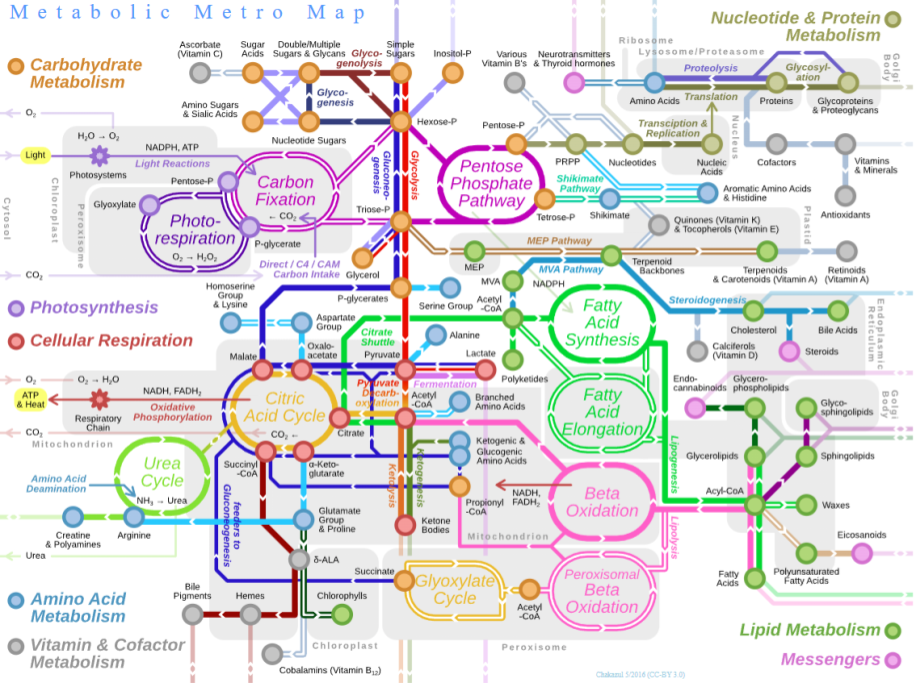
Metabolic networks are not tangled webs. Their architecture is hierarchically modular: tightly linked modules nest within larger modules, all organized around a small connective core (Ravasz et al. 2002). Architectures like this arise when networks expand by attachment, each new pathway bolting onto machinery that already exists. And once a dozen downstream pathways depend on an upstream reaction, that reaction is frozen in place; changing it breaks everything built on top. Wimsatt (2007) calls this generative entrenchment. Entrenchment gives the network a readable stratigraphy. Deeply embedded core chemistry should tend to be older than dependent peripheral pathways. We will meet the same logic again when we explore the ribosome’s history from its onion-like layers. 

All living things rely on energy metabolism to fuel themselves and anabolism to build up complex organics. The differences reside where the carbon comes from. Autotrophs use carbon fixation to build biomass from inorganic carbon such as CO2. Heterotrophs obtain reduced carbon from the environment, and rely on catabolism to break down the complex organics in their diet. 

The modern biosphere rests on an autotrophic foundation. Nearly all carbon enters through the fixation of CO2. Life does not depend significantly on extraterrestrial, atmospherically or geologically produced organics. But on the Hadean Earth, impact delivery supplied organics at a far higher rate. Oparin and Haldane’s original vision of primordial soup presumed a heterotrophic origin. So which was it? Did the first life eat chondrites or fix carbon? 

Two converging lines of evidence suggest fixation. The first comes from genes and energetics. Weiss et al. (2016) traced 355 gene families back to LUCA and recovered the profile of an anaerobic, H2-dependent autotroph. Phylogenetic reconstructions are often contested. But Wimmer et al. (2021) computed the thermodynamics of LUCA’s ~400 core reactions and found that roughly 96% run exergonically under H2-rich anoxic conditions. The genes describe an autotroph, and the metabolism they encode fits an autotroph’s environment.

The second line of evidence applies our stratigraphy. Catabolism sits at the periphery. Major catabolic pathways characteristically converge on the universal anabolic core. Moreover, the substrates it digests are sugars, lipids, and proteins: the characteristic products of anabolism (Schönheit, Buckel & Martin 2016). The enzyme record concurs. The ancestral fructose-bisphosphate enzyme of archaea is locked into the gluconeogenic direction, marking glycolysis as a later retrofit (Say & Fuchs 2010). 

Taken together, these suggest that anabolism came first. The first life was likely autotrophic.

Carbon fixation places specific requirements on the environment. It requires both CO2 and a continuous electron supply. Candidate electron donors (reductants) include H2, Fe(II), and H2S. Reductant and carbon co-delivery denotes the requirement that electron donors and inorganic carbon arrive together, continuously, at rates sufficient to sustain fixation.

Anabolic metabolism synthesizes thousands of biological molecules. The stratigraphy points inward: the oldest chemistry of all should sit at the very center of the network. Smith and Morowitz (2004) identify it. Eleven carboxylic acids form a universal anabolic core.

With a handful of glycine-related exceptions, all biosynthesis radiates from five of these acids. Acetate seeds the lipids; pyruvate the sugars and the alanine-family amino acids; oxaloacetate the aspartate family, and through aspartate the pyrimidines; α-ketoglutarate the glutamate family; succinyl-CoA the pyrroles. (Purines are the untidy exception, assembled from glycine, aspartate, glutamine, and the same C1 chemistry owned by the WL pathway) These are the pillars of anabolic metabolism

The entire biosphere uses seven carbon fixation pathways (CBB, rTCA, WL, 3-HP, 3-HP/4-HB, DC/4-HB, and roTCA). Which of these was used by LUCA? 

You may recall learning about the tricarboxylic acid (TCA) cycle (aka Krebs cycle) at school. In modern organisms, this cycle is catabolic. For decades that was its only known direction. But Evans et al (1966) and Shiba et al (1985) discovered it also runs in the reverse direction. This rTCA cycle is an autotrophic engine of carbon fixation. The eleven carboxylic acids are precisely the universal anabolic core. It is a strong candidate for the seed of protometabolism. 

Several steps of any fixation pathway are endergonic (thermodynamically dysfavored) under ordinary conditions. Modern cells pay for these steps with ATP hydrolysis. A protometabolism has no ATP. The environment itself must pay. Thermodynamic drive denotes the requirement that environmental chemistry makes the overall pathway favorable without modern energy currencies like ATP.

We have identified the rTCA cycle by reading the network’s stratigraphy. Comparative biology provides another glimpse. Consider organisms that are anaerobic and chemoautotrophic. In archaea, these are the methanogens; in bacteria the acetogens. What do they have in common? 

Both methanogens and acetogens rely on the Wood-Ljungdahl (WL) pathway (aka acetyl-CoA pathway). WL is in fact the only carbon-fixation pathway found in both bacteria and archaea. Weiss et al (2016) place WL in LUCA itself. WL is also thermodynamically unique. Every other fixation pathway runs uphill and is financed with ATP. The Calvin cycle spends roughly nine ATP per pyruvate; rTCA is among the cheapest. WL runs downhill. Under anoxic conditions with H2 as the electron donor, the overall reaction is exergonic, releasing roughly 100 kJ/mol. Acetogens and methanogens exploit this: the same pathway that builds their biomass also charges their membranes and makes their ATP.  A cell running WL on a H2 supply occupies what Everett Shock called a “free lunch you are paid to eat.” WL is the only fixation chemistry that could have paid its own way. 

Finally, methanogens and acetogens also share a second piece of machinery: flavin-based electron bifurcation. The problem it solves is that reducing CO₂ requires electrons at potential lower than H₂ itself can supply. Bifurcation takes an electron pair from a mid-potential donor and splits it: one electron falls to a high-potential acceptor, and the energy released pays for lifting the other onto low-potential ferredoxin, the reductant that carbon fixation demands. Its distribution across both domains marks it as ancient (Buckel & Thauer 2013).

These two engines have complementary strengths and weaknesses. rTCA contains the entire anabolic core, and it is autocatalytic. But it runs uphill. WL has the right energetics: it is the only chemistry that runs downhill. But it is a linear, non-autocatalytic path, and hence cannot auto-amplify. Braakman and Smith (2013) place a fused WL-rTCA network at the base of the tree. For now, we will treat these fixation pathways as complementary halves of one machine.

Both WL and rTCA are now executed by enzymes. But buried inside many of these proteins are metal-sulfur cofactors, and these are often the catalytically active sites. Ferredoxin contains cubanes whose geometry resembles motifs found in  the mineral greigite (via its precursor mackinawite). The nickel-iron-sulfur cluster at the heart of CO dehydrogenase and acetyl-CoA synthase likewise resembles violarite. Zhao et al. (2022) quantified these cofactor-mineral correspondences. These structural correspondences hint at evolutionary continuity. Russell and Martin (2004) argue that these catalytic sites are mineral fossils, and the surrounding protein is later packaging around an ancient inorganic core. 

Metabolism-first envisions a non-enzymatic protometabolism. Geochemical continuity suggests the earliest catalysts were mineral. But modern enzymes accelerate reactions by factors up to 10^17. Without them, most reactions proceed at negligible rates. Kinetic accessibility denotes the experimental requirement that mineral, metal, or small-molecule catalysts sit in the flow path and drive the key reactions at meaningful rates. 

Vigorous flow solves one problem and creates another. The same throughput that delivers reductant and exports waste can wash a network’s working parts away faster than the chemistry regenerates them. A pathway turns on a characteristic timescale, and its intermediates must survive long enough to complete the loop. Intermediate retention denotes the requirement that residence times exceed network turnover times.

The deepest layer of the network has another striking property. If we abstract away the modern enzymes, cofactors, and carrier groups that now mediate it, the carbon skeletons of WL and rTCA contain only carbon, hydrogen and oxygen. These skeletons are strictly a CHO metabolism. Nitrogen is not needed to construct this central carbon framework. It seems to have entered later, converting pre-existing carbon skeletons into amino acids and the broader CHON metabolism (Braakman & Smith 2013).  Phosphate may show a similar pattern: Goldford et al. (2017) reconstructed a plausible ancient metabolic network with little dependence on phosphate, although Tian et al. (2019) contest how far that inference can be pushed.  This is compatible with de Duve (1991)’s hypothesis that thioesters (like acetyl-CoA) served as an energy currency predecessor of ATP. 

The resulting picture is one of elemental expansion: a CHO carbon-skeleton core, followed by nitrogen incorporation and increasingly phosphate-dependent chemistry. This ordering is naturally compatible with metabolism-first. If RNA came first, despite already requiring fixed nitrogen and phosphate, it becomes less obvious why the deepest metabolic layers should preserve a simpler elemental architecture. 

A Scorecard For Habitat

We have generated twenty requirements.

Universal (11)

  • Sustained free-energy flux. Continuous or recurrent throughput maintaining far-from-equilibrium chemistry.
  • Chemical selectivity. Flux channeled toward targets, against the combinatorial tar.
  • Provenance. Feedstocks and catalysts arise or arrive naturally.
  • Reactant concentration. Feedstocks reach reaction-viable concentrations.
  • Material flux. Energy and material in, waste out, spent material recycled.
  • Product retention. Useful products stay long enough to react again (in creative tension with material flux).
  • Net production. Target made faster than destroyed.
  • Condition compatibility. Incompatible reactions confined to microenvironments that exchange products realistically.
  • Process continuity. Each chemical step connects in geochemically plausible way, without artificial laboratory techniques.
  • Habitat persistence. Eden either outlasts, or recurs frequently.
  • Localization. Products must preferentially benefit the systems that produce them, rather than diffusing to competitors. 

Genetics-first (5)

  • Bioavailable nitrogen. Reactive C–N precursors.
  • Bioavailable phosphate. Soluble, concentrated phosphate despite mineral lock-up.
  • Monomer activation. Free energy stored or coupled so phosphodiester bonds can form.
  • Polymer elongation. Bond formation is efficient and repeatable to functional lengths.
  • Template reset. Duplexes separate non-destructively for the next round.

Metabolism-first (4)

  • Reductant and carbon co-delivery. Electron donors and CO₂ arrive together, continuously.
  • Thermodynamic drive. The environment pays for endergonic chemistry without ATP.
  • Kinetic accessibility. Non-enzymatic catalysts must drive key reactions at meaningful rates.
  • Intermediate retention. Residence times exceed network turnover times.

Next post, we will use this scorecard to grade specific hypotheses from both camps. See you then!

References

  • Braakman & Smith (2013). The Compositional and Evolutionary Logic of Metabolism.
  • Buckel & Thauer (2013). Energy Conservation via Electron-Bifurcating Ferredoxin Reduction and Proton/Na⁺-Translocating Ferredoxin Oxidation.
  • Butlerov (1861). Formation Synthétique d’une Substance Sucrée.
  • de Duve (1991). Blueprint for a Cell: The Nature and Origin of Life.
  • Evans, Buchanan & Arnon (1966). A New Ferredoxin-Dependent Carbon Reduction Cycle in a Photosynthetic Bacterium.
  • Gianni et al. (2026). A Small Polymerase Ribozyme That Can Synthesize Itself and Its Complementary Strand.
  • Goldford, Hartman, Smith & Segrè (2017). Remnants of an Ancient Metabolism without Phosphate.
  • Hud et al. (2013). The Origin of RNA and “My Grandfather’s Axe.”
  • Kruger et al. (1982). Self-Splicing RNA: Autoexcision and Autocyclization of the Ribosomal RNA Intervening Sequence of Tetrahymena.
  • Mateo-Marti et al. (2019). Pyrite-Induced UV-Photocatalytic Abiotic Nitrogen Fixation: Implications for Early Atmospheres and Life.
  • Nissen et al. (2000). The Structural Basis of Ribosome Activity in Peptide Bond Synthesis.
  • Pitsch et al. (1995). Mineral Induced Formation of Sugar Phosphates.
  • Ravasz et al. (2002). Hierarchical Organization of Modularity in Metabolic Networks.
  • Russell & Martin (2004). The Rocky Roots of the Acetyl-CoA Pathway.
  • Say & Fuchs (2010). Fructose 1,6-Bisphosphate Aldolase/Phosphatase May Be an Ancestral Gluconeogenic Enzyme.
  • Schönheit, Buckel & Martin (2016). On the Origin of Heterotrophy.
  • Shiba et al. (1985). The CO₂ Assimilation via the Reductive Tricarboxylic Acid Cycle in an Obligately Autotrophic, Aerobic Hydrogen-Oxidizing Bacterium, Hydrogenobacter thermophilus.
  • Smith & Morowitz (2004). Universality in Intermediary Metabolism.
  • Tian et al. (2019). Phosphates as Energy Sources to Expand Metabolic Networks.
  • Toner & Catling (2020). A Carbonate-Rich Lake Solution to the Phosphate Problem of the Origin of Life.
  • Weiss et al. (2016). The Physiology and Habitat of the Last Universal Common Ancestor.
  • White (1976). Coenzymes as Fossils of an Earlier Metabolic State.
  • Wimmer et al. (2021). Energy at Origins: Favorable Thermodynamics of Biosynthetic Reactions in the Last Universal Common Ancestor.
  • Wimsatt (2007). Re-Engineering Philosophy for Limited Beings: Piecewise Approximations to Reality.
  • Yadav et al. (2020). Chemistry of Abiotic Nucleotide Synthesis.
  • Zhao et al. (2022). Quantifying Mineral-Ligand Structural Similarities: Bridging the Geological World of Minerals with the Biological World of Enzymes
A Portrait of LUCA

Part Of: Biology sequence
Content Summary: 3000 words, 15 min read

The Basic Facts of Abiogenesis

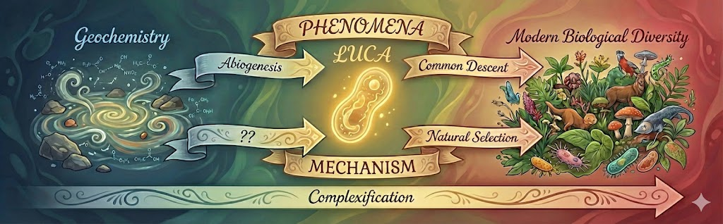
From the geochemistry of the early Earth, life emerged. The abiogenesis phenomenon is interesting in at least two contexts:

First, it is one of the most difficult unsolved scientific problems in the 21st century. Common descent describes how all of the marvelous diversity of biology stem from a single source: a single celled organism called the Last Universal Common Ancestor (LUCA). We have a clear mechanistic understanding for how this complexification was possible: evolution by natural selection

But natural selection relies on the machinery of genetic inheritance to produce complexity. How was it possible to create the sophisticated nanomachinery of LUCA (e.g., ATP synthase) before natural selection took effect? What other process besides natural selection can produce complexification?

Second, abiogenesis research is relevant to questions in astrobiology:

Could extraterrestrial life have begun much earlier? 

  • Gen 1 stars (born 13.5-13 Ga) had no exoplanets because the heavy elements required for planetary cores didn’t exist (supernova nucleosynthesis arrived later). 
  • Gen 2 stars (born 13-10 Ga) may have been able to support life, but these exoplanets were small, terrestrial, and less metallic – unable to furnish geomagnetism nor plate tectonics. 
  • Gen 3 stars (born 10-0 Ga) can support life. Exoplanets in this era now include gas giants, and are highly metallic. Geomagnetism protects us from UV radiation, and plate tectonics promote mineral diversity. 

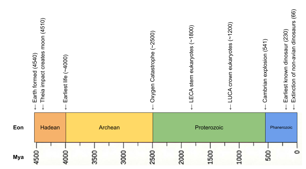
Is abiogenesis easy or hard? The Earth was born 4.6 Ga, with the Theia impactor at 4.54 Ga creating the moon and the Moneta impactor at 4.51 Ga providing siderophilic veneer. Despite such impacts, zircon evidence now suggests a cool early earth, with oceans appearing as early as 4.4 Ga. Critically, our evidence for life arrives very early (Isua banded-iron formations at 3.8 Ga, enriched carbon-12 in zircon graphite at 4.1 Ga). Abiogenesis occurred only ~500 million years after the sterilizing impact of Moneta! Speed is evidence of ease.

If the universe has billions of potentially habitable planets, why haven’t we found any aliens? One explanation to the Fermi Paradox is the Great Filter – some incredibly difficult barrier that prevents life from becoming spacefaring. The scary part is we don’t know where this filter is: behind us (we got incredibly lucky to make it this far) or ahead of us (something typically destroys civilizations before they can spread across the galaxy). If abiogenesis is indeed easy, this might mean the Great Filter is ahead of us.

LUCA from Paleobiogeography

To understand the journey of abiogenesis, we must first understand the destination. What do we know about LUCA?

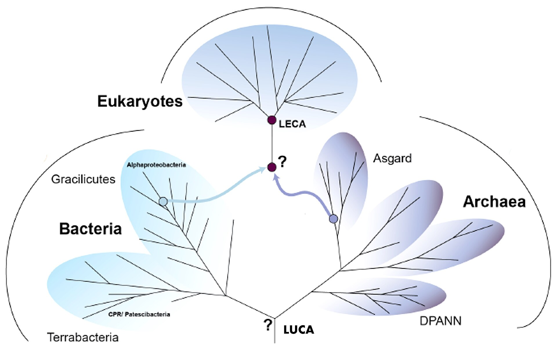
The history of life constrains our search. Two domains of simple life (prokaryotes) emerged in the Hadean: bacteria and archaea. But eukaryotes (complex life) emerged much later, as a result of endosymbiosis between the two families. 

Life was microbial for the first 80% of Earth’s history. But in 1.0 Ga, multicellularity was invented. Starting at that time, multicellularity was invented multiple times, but it only really took off in crown group eukaryotes. 

LUCA must have been anaerobic. For the first half of Earth’s history, oxygen was locked in water and rocks – there was no free oxygen in the atmosphere. Only when photosynthesis caused the Oxygen Catastrophe in 2.4 Ga did atmospheric oxygen go from 0 to 10%. 

LUCA is simple (prokaryotic), microbial (unicellular), and anaerobic.

LUCA from Phylogenetics

We can learn more about LUCA from genetic analyses. 

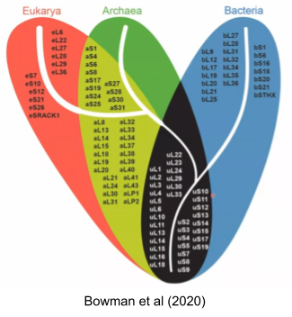
Genes conserved across all species constitute what is called the Universal Gene Set of Life (UGSL), and consists of less than 100 genes (Harris et al 2003). Not surprisingly, the UGSL is dominated by translation-related genes. Here are those ribosomal genes in black:

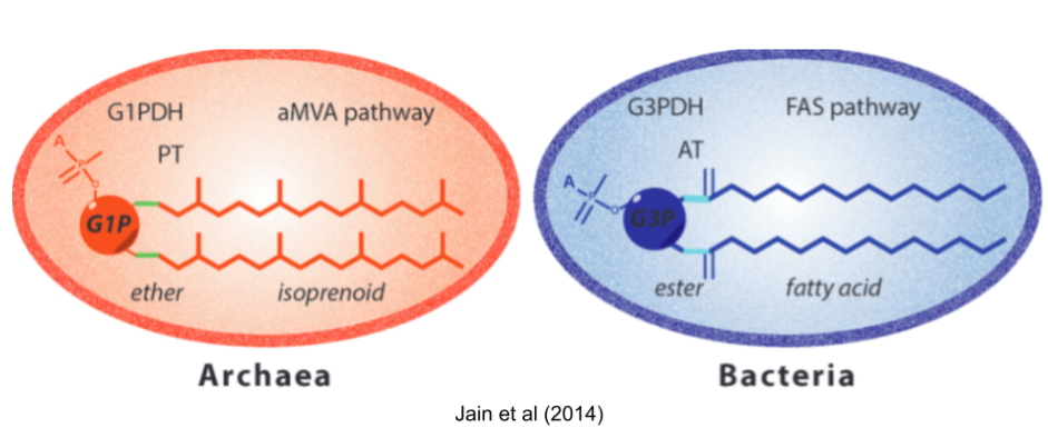
Many differences between archaea and bacteria arose after they diverged. But some differences are more troubling. First among these is the Lipid Divide. Both domains build cells with the phospholipid bilayer membranes, so it is natural to suspect that LUCA had a similar coat. But almost all biochemical details are mirrored! They use different glycerol backbones, different hydrophobic chains (isoprenoid vs fatty acids), different links to those chains (ether vs ester), and different biosynthetic pathways (FAS+AT vs aMVA+PT). 

There are three major theories for the lipid composition of LUCA:

  • Heterochiral theories. LUCA had both lipid biochemistries available. Heterochiral membranes were recently found to be viable (Caforio et al 2018). 
  • Thermoreduction theories. Many archaea are adapted to extreme environments. So LUCA had a bacterial phospholipid, and the more robust archaeal lipids were derived to support more extreme niches.
  • Protocompartment theories. LUCA didn’t use phospholipids at all! It used a simple fatty acid membrane, or coacervate droplets, or mineral pores to achieve compartmentalization.

Another divergence is even more troubling: bacteria and archaea use completely different DNA replicase proteins (Forterre et al 2013). 

Neither divide has a satisfying resolution. Each of the three lipid hypotheses faces serious objections, and the DNA replicase situation is arguably worse: there is no consensus account for how two non-homologous replication machineries could descend from a single ancestor, which has led some (e.g., Forterre 2006) to argue that DNA itself was a viral invention acquired independently by the bacterial and archaeal lineages. Any portrait of LUCA that papers over these divides is overconfident.

LUCA from Biochemistry

At the atomic level, organisms are built with CHNOPS: Carbon, Hydrogen, Nitrogen, Oxygen, Phosphorous, and Sulfur. 

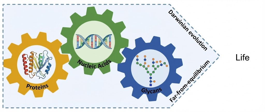
At the molecular level, life is composed of three biopolymers.

  • Glycans are made out of monosaccharides (e.g., glucose). 
  • Proteins are made out of amino acids.
  • Nucleic acids are made out of nucleotides

Most of our discussion will center on proteins and nucleic acids. Their constituents are themselves large, complex molecules. These monomers are built on an unchanging backbone and a variable side chain. For nucleotides, there are 4 available side chains (purine and pyrimidine nitrogenous bases). For amino acids, there are 20 available side chains (nonpolar, polar-uncharged, polar-positive, polar-negative R groups).

Organic polymers like polyesters aren’t particularly flexible. But biopolymers manifest extreme functional sophistication. And the polyfunctionality of nucleic acids and glycans must not be understated (Matange et al 2025).

Biopolymers also exhibit functional interdependence. Condensation of nucleotides is catalyzed by proteins, and condensation of amino acids is catalyzed by RNA. Biopolymers are heterocomplementary: proteins can recognize and bind to proteins, DNA, polyglycans, and small molecules. Nonbiological organic polymers do not manifest heterocomplementarity. 

LUCA from Microbiology

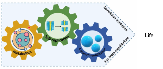
Another way to approach LUCA is to catalog biological universals: mechanisms shared by all life forms in existence. These universals can be organized in three categories: self-replication, metabolism, and compartmentalization. Let’s discuss each in turn.

The central genius of life was the discovery of proteins. By chaining amino acids together in long biopolymers, these polypeptides fold into arbitrary shapes. This invention is so powerful because in chemistry, structure determines function: arbitrary shapes unlock myriad potential behaviors. Proteins can form fibers, motors, containers, transporters, sensors, signals, optical devices, adhesives, pores, brushes, and pumps. 

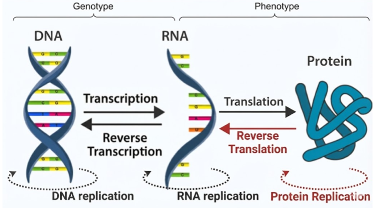
Proteins aren’t synthesized randomly – they are produced by template. Nucleotides combine together in long biopolymers known as nucleic acids. Double-stranded DNA is copied into single-stranded mRNA via the process of transcription. Then, during protein synthesis in the ribosome, codons (RNA triplets) specify which amino acids to attach in which order. This process of translation is defined by a codon-amino acid map known as the genetic code

A gene is simply a patch of RNA that completely specifies a particular protein sequence. Your genome (genotype) is nothing more than a recipe for a proteome (phenotype). When philosophers speak of an innate desire to survive, that motivation must be carried by proteins. Natural selection operates on protein design. Nothing more and nothing less.

The Central Dogma describes the flow of information in biopolymers. The black arrows are allowed processes; the red arrows are not observed. Proteins cannot replicate because they are incapable of base pairing. Once information gets into a protein, it cannot get out again!

Why is life so fixated on proteins? To better understand this, it helps to consider metabolism. This is a chemical reaction network which provides two basic functions: 

  1. Catabolism (“energy metabolism”), a destructive process which breaks down complex compounds. This prominently includes pathways of cellular respiration, a controlled version of combustion in which glucose is slowly converted into carbon dioxide, water, and energy. 
  2. Anabolism (“carbon metabolism”), a constructive process which biosynthesizes new organic compounds. This includes pathways of carbon fixation (like Acetyl-CoA), which converts simple inorganic carbon dioxide into complex organics.

Enzymes are protein-based catalysts that reduce the activation energy of thermodynamically favorable (exergonic) reactions, speeding them up by many orders of magnitude. Some metabolic steps, however, are thermodynamically disfavorable (endergonic) and will not proceed spontaneously. Enzymes handle these by coupling them to a favorable reaction, making the combined process exergonic. The enzyme then catalyzes that coupled reaction in the usual way — by lowering its activation energy.

The 20 amino acids have a limited chemical repertoire; cofactors extend it — enabling electron transfer, redox chemistry, and group transfers that amino acid side chains cannot perform alone. There are two categories of cofactors: metal ions (e.g., Mg²⁺, and Fe²⁺), and organic molecules (i.e., coenzymes), many of which are derived from B vitamins (e.g., NAD). Without its cofactor, an enzyme (called an apoenzyme) is typically inactive. The complete, functional assembly is the holoenzyme.

Finally, while the Central Dogma traditionally depicts a linear flow of information from DNA to RNA to Protein, metabolism reveals that this dogma is actually a loop. Proteins are not just passive end-products; they are the active machinery required to synthesize and maintain the very DNA and RNA that encode them, creating a self-sustaining cycle of synthesis and regulation.

Modern metabolism and self-replication does not occur in an undifferentiated “primordial soup”. They occur inside impermeable membranes made of phospholipids. 

Compartmentalization does a lot of heavy lifting at once: it shields nucleic acids from genetic parasites, buffers the system against environmental stress, and locally concentrates enzymes and substrates to speed reactions. By keeping metabolites and genetic material from simply diffusing away, it preserves hard-won products and information. Selective, protein-based gates regulate traffic—letting in foodstuffs, exporting waste—and can couple chemiosmosis to maintain a strong proton-motive force (≈3 pH units and ~200 mV), effectively a “cellular battery” that powers metabolic work. Finally, a stable compartment provides the physical unit that can reliably copy itself and propagate success via binary fission.

LUCA from Virology

Previous sections reconstructed LUCA as a cell. But modern oceans contain ten virions for every microbe. Viruses coevolve with cells, outnumber them, and may even predate them. Any reconstruction of early life that ignores them is incomplete.

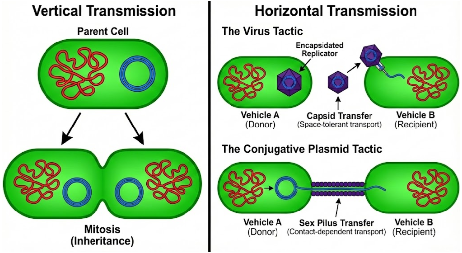
Once inside the cell, virulent viruses initiate the lytic cycle. Their genes hijack the host cell’s machinery to make more copies of themselves, ultimately rupturing the membrane and spilling newly-minted virions into the environment. They rely on horizontal transmission, in contrast to chromosomes which rely on vertical transmission via mitosis.  

Viruses are not the only mobile genetic element (MGE) using horizontal transmission. Cells can contain small (often circular) nucleic acid outside of the chromosomes. These plasmids don’t kill the cell to transfer their DNA, but instead use conjugative sex pili to copy themselves into neighboring cells. Plasmid genetic material can be more similar to viruses than the chromosome. Some plasmids and viruses differ by no more than a capsid gene (Krupovic & Bamford 2010).

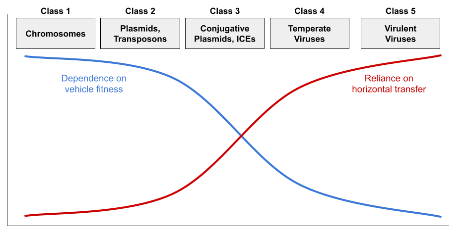
But virulence and conjugation are extremes. While virulent viruses are indifferent to cellular fitness, temperate viruses benefit from vertical transmission via the lysogenic cycle. They are thus less pathogenic. Some plasmids cannot construct the sex pilus and are capable of horizontal transmission only rarely. Jalasvuori (2012) shows that nucleic acids can be organized into a continuum:

This framework explains the distribution of replicator properties:

  • Class 3-5 all sense damage to the host cell, and initiate horizontal transfer when they detect vehicle stress. For example, herpesviruses reactivate from latency under host stress, producing cold sores.
  • Class 1 retains the core genome (e.g., DNA replication). Class 2-3 retain the accessory genome (e.g., virulence, antibiotic resistance).
  • Class 1-5 all retain addiction modules (a.k.a., MGE stabilization modules) like the toxin-antitoxin (TA) system (Mendoza-Guido & Rojas-Jimenez 2025). Many plasmids produce both a toxin and the antitoxin. Since the toxin has a longer half-life, loss of the plasmid entails death of the host. The restriction-modification (RM) system works in a very similar way (Kobayashi 2001).

There are three hypotheses for the origin of viruses:

  • The regression hypothesis claims that viruses are cells that progressively lost genetic information in their journey towards obligate parasitism.
  • The escape hypothesis claims that viruses originate from MGEs that gained increasingly sophisticated methods of horizontal transfer.
  • The virus-first hypothesis claims that viruses predate LUCA, originating from the primordial pool of replicators prior to the evolution of cells.

Dependent niches incentivize genome reduction. Mitochondria have transferred many genes to their host cells’ nuclei (Andersson & Kurland 1998), and parasitic bacteria like Rickettsia have shed much of theirs (Diop et al 2019). As obligate parasites, viruses should face the same reductive pressure — but what if they weren’t always parasitic? The discovery of giant viruses (in the phylum Nucleocytoviricota), with the first known translation-related machinery in a virus, was a revelation. In the spirit of the regression hypothesis, Boyer et al (2010) described them as living fossils of this fourth domain. But, while the relationship between reduction and parasitism is strong, recent phylogenetic work (Monttinen et al 2021) does not support this hypothesis.

The escape hypothesis accounts for some viral genes – particularly those encoding capsid proteins – which have clear cellular homologs. But viral hallmark genes, especially those involved in replication, are shared across diverse viral lineages yet absent from cellular genomes (Koonin et al 2006). If these genes escaped from cells, their cellular homologs should exist. Krupovic et al (2019) propose a chimeric origin that reconciles the escape and virus-first views. They argue that structural genes were captured from hosts, but replicator genes descend from primordial self-replicating elements that predate cells. 

Theoretical models reinforce this view — selfish genetic elements arise inevitably in any replicator system, suggesting that genetic parasites have been components of life from the very beginning. Before replicators evolved error correction mechanisms, early replicators also faced a hard physical constraint known as Eigen’s error threshold: RNA replication error rates impose an upper bound on genome size. Viroids, the simplest known replicators at ~300 nucleotides, sit near this boundary. If the chimeric model is correct and viral replicator genes descend from primordial self-replicating elements, viroids may be the closest living relatives of those elements. Their structural simplicity, their lack of protein-coding capacity, and the recent discovery of viroid-like circular RNAs across diverse environments (Lee et al 2023) are all consistent with deep ancestry.

Looking Beyond the Root

The portrait above shows LUCA as anaerobic, prokaryotic, protein-dependent, chromosomally organized, besieged by viruses. But every feature of that portrait is also a choice made from a menu of alternatives that were never taken:

  • Alternative codes. Of ~500 amino acid species, only 20 are included in the genetic code, even though codons could distinguish up to 64. Central metabolites like ornithine, GABA, and β-alanine are biosynthesized but never translated.
  • Alternative replicator backbones. 5-carbon sugars (ribose, deoxyribose) are a strange choice for a nucleic acid backbone (Eschenmoser 1999). Chemists have built alternative replicators from 4-carbon sugars (TNA) and 3-carbon sugars (GNA).
  • Alternative protein backbones. Proteins are built from α-amino acids, but foldamers made from β, γ, and δ-amino acids can be more resistant to proteolysis and heat denaturation than their α-counterparts (Gellman 1998).

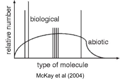
McKay (2004) captures this puzzle visually: nonbiological chemistry produces smooth distributions of organic molecules, but life uses only a sparse set of spikes against that background.


Each of these alternatives works better than what life uses, on some axis. So the interesting question isn’t whether LUCA could have been different; it’s why it wasn’t. Why haven’t we found shadow biospheres running on TNA, or β-peptide proteomes, or 34-amino-acid codes? Two possibilities: either we haven’t looked hard enough, or these choices were frozen so early and so deeply that no later lineage could back out of them. Both answers require understanding what happened before LUCA: the evolution of the ribosome, the freezing of the code, the crystallization of a chromosome out of competing replicators.

Beyond the root of the tree of life lies the origin. That’s the subject of our next post.

References

  • Andersson & Kurland (1998). Reductive evolution of resident genomes
  • Bowman et al (2020). Root of the Tree: The Significance, Evolution, and Origins of the Ribosome
  • Boyer et al (2010). Phylogenetic and Phyletic Studies of Informational Genes in Genomes Highlight Existence of a 4th Domain of Life Including Giant Viruses
  • Caforio, A., et al. (2018). “Converting Escherichia coli into an archaebacterium with a hybrid heterochiral membrane.”
  • Diop et al (2019). Paradoxical evolution of rickettsial genomes
  • Eschenmoser (1999). Chemical etiology of nucleic acid structure.
  • Forterre (2006). The origin of viruses and their possible roles in major evolutionary transitions.
  • Forterre et al (2013) Origin and Evolution of DNA and DNA Replication Machineries
  • Gellman (1998). Foldamers: A manifesto.
  • Harris et al (2003). The genetic core of the universal ancestor. 
  • Jain et al (2014). Biosynthesis of archaeal membrane ether lipids
  • Jalasvuori (2012). Vehicles, replicators, and intercellular movement of genetic information: evolutionary dissection of a bacterial cell. 
  • Koonin et al (2006). The ancient virus world and evolution of cells. 
  • Kobayashi (2001). Behavior of restriction–modification systems as selfish mobile elements and their impact on genome evolution.
  • Krupovic et al (2019). Origin of viruses: primordial replicators recruiting capsids from hosts.
  • Krupovic & Bamford (2010). Order to the viral universe
  • Lee et al (2023). Mining metatranscriptomes reveals a vast world of viroid-like circular RNA
  • Matange et al (2025). Biological polymers: evolution, function, and significance.
  • McKay (2004). What Is Life—and How Do We Search for It in Other Worlds?
  • Mendoza-Guido & Rojas-Jimenez (2025). Beyond plasmid addiction: the role of toxin-antitoxin systems in the selfish behavior of mobile genetic elements. 
  • Monttinen et al (2021). The genomes of nucleocytoplasmic large DNA viruses: viral evolution writ large

An Introduction To Natural Selection

Part OfDemystifying Life sequence
Followup To: Population Genetics
Content Summary: 1400 words, 14 min read

How Natural Selection Works

Consider the following process:

  1. Organisms pass along traits to their offspring.
  2. Organisms vary. These random but small variations trickle through the generations.
  3. Occasionally, the offspring of some individual will vary in a way that gives them an advantage.
  4. On average, such individuals will survive and reproduce more successfully.

This is how favorable variations come to accumulate in populations.

Let’s plug in a concrete example. Consider a population of grizzly bears that has recently migrated to the Arctic.

  1. Occasionally, the offspring of some grizzly bear will have a fur color mutation that renders their fur white.
  2. This descendent will on average survive and reproduce more successfully.

Over time, we would expect increasing numbers of such bears to possess white fur.

Biological Fitness Is Height

The above process is straightforward enough, but it lacks a rigorous mathematical basis. In the 1940s, the Modern Evolutionary Synthesis enriched natural selection by connecting it to population genetics, and its metaphor of Gene-Space. Recall what we mean by such a landscape:

  • A Genotype Is A Location.
  • Organisms Are Unmoving Points
  • Birth Is Point Creation, Death Is Point Erasure
  • Genome Differences Are Distances

Onto this topography, we identified the following features:

  • A Species Is A Cluster Of Points
  • Species Are Vehicles
  • Genetic Drift is Random Travel.

In order to understand how natural selection enriches this metaphor, we must define “advantage”. Let biological fitness refer to how how many fertile offspring an individual organism leaves behind. An elephant with eight grandchildren is more fit than her neighbor with two grandchildren.

Every organism achieves one particular level of biological fitness. Fitness denotes how well-suited an organism is to its environment. Being a measure of organism-environment harmony, we can view fitness as defined for every genotype. Since we can define some number for every point in gene-space, we have license to introduce the following identification:

  • Biological Fitness Is Height

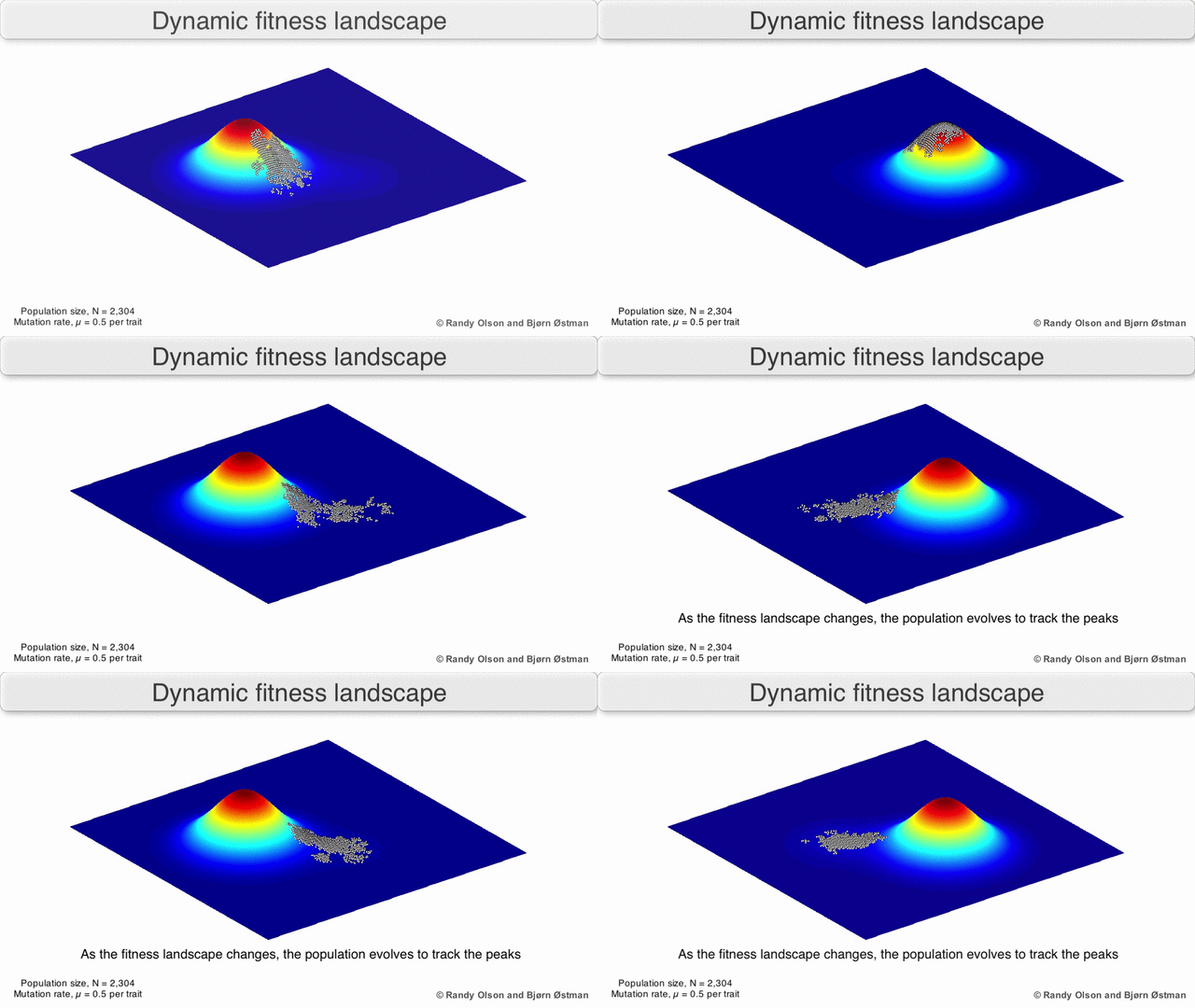
Here is one possible fitness landscape (image credit Bjørn Østman).

Natural Selection- Fitness Landscape (1)

We can imagine millions of alien worlds, each with its own fitness landscape. What is the contours of Earth’s?

Let me gesture at three facts of our fitness landscape, to be elaborated next time:

  • The total volume of fitness is constrained by the sun. This is hinted at by the ecological notion of carrying capacity.
  • Fitness volume can be forcibly taken from one area of the landscape to another. This is the meaning of predation.
  • Since most mutations are harmless, the landscape is flat in most directions. Most non-neutral mutations are negative, but some are positive (example).

Natural Selection As Mountain Climbing

A species is a cluster of points. Biological fitness is height. What happens when a species resides on a slope?

The organisms uphill will produce comparatively more copies of themselves than those downhill. Child points that would have been evenly distributed now move preferentially uphill. Child points continue appearing more frequently uphill. This is locomotion: a slithering, amoeba-like process of genotype improvement.

NaturalSelection_Illustration

We have thus arrived at a new identification:

  • Natural Selection Is Uphill Locomotion

As you can see, natural selection explains how species gradually become better suited to their environment. It is a non-random process: genetic movement is in a single direction.

Consider: ancestral species of the camel family originated in the American Southwest millions of years ago, where they evolved a number of adaptations to wind-blown deserts and other unfavorable environments, including a  long neck and long legs. Numerous other special designs emerged in the course of time: double rows of protective eyelashes, hairy ear openings, the ability to close the nostrils, a keen sense of sight and smell, humps for storing fat, a protective coat of long and coarse hair (different from the soft undercoat known as “camel hair”), and remarkable abilities to take in water (up to 100 liters at a time) and do without it (up to 17 days).

Moles, on the other hand, evolved for burrowing in the earth in search of earthworms and other food sources inaccessible to most animals. A number of specialized adaptations evolved, but often in directions opposite to those of the camel: round bodies, short legs, a flat pointed head, broad claws on the forefeet for digging. In addition, most moles are blind and hard of hearing.

The mechanism behind these adaptations is selection, because each results in an increase in fitness, with one exception. Loss of sight and hearing in moles is not an example of natural selection, but of genetic drift: blindness wouldn’t confer any advantages underground, but arguably neither would eyesight.

Microbiologists in my audience might recognize a strong analogy with bacterial locomotion. Most bacteria have two modes of movement: directed movement (chemotaxis) when its chemical sensors detect food, and a random walk when no such signal is present. This corresponds with natural selection and genetic drift, respectively.

Consequences Of Optimization Algorithms

Computer scientists in my audience might note a strong analogy to gradient descent, a kind of algorithm. In fact, there is a precise sense in which natural selection is an optimization algorithm. In fact, computer scientists have used this insight to design powerful evolutionary algorithms that spawn not one program, but thousands of programs, rewarding those with a comparative advantage. Evolutionary algorithms have proven an extremely fertile discipline in problem spaces with high dimensionality. Consider, for example, recent advances in evolvable hardware:

As predicted, the principle of natural selection could successfully produce specialized circuits using a fraction of the resources a human would have required. And no one had the foggiest notion how it worked. Dr. Thompson peered inside his perfect offspring to gain insight into its methods, but what he found inside was baffling. The plucky chip was utilizing only thirty-seven of its one hundred logic gates, and most of them were arranged in a curious collection of feedback loops. Five individual logic cells were functionally disconnected from the rest— with no pathways that would allow them to influence the output— yet when the researcher disabled any one of them the chip lost its ability to discriminate the tones…

It seems that evolution had not merely selected the best code for the task, it had also advocated those programs which took advantage of the electromagnetic quirks of that specific microchip environment. The five separate logic cells were clearly crucial to the chip’s operation, but they were interacting with the main circuitry through some unorthodox method— most likely via the subtle magnetic fields that are created when electrons flow through circuitry, an effect known as magnetic flux. There was also evidence that the circuit was not relying solely on the transistors’ absolute ON and OFF positions like a typical chip; it was capitalizing upon analogue shades of gray along with the digital black and white.

In gradient descent, there is a distinction between global optima and local optima. Despite the existence of an objectively superior solution, the algorithm cannot get there due to its fixation with local ascent.

Natural Selection- Local vs. Global Optima

This distinction also features strongly in nature. Consider again our example of camels and moles:

Given such a stunning variety of specialized differences between the camel and the mole, it is curious that the structure of their necks remains basically the same. Surely the camel could do with more vertebrae and flex in foraging through the coarse and thorny plants that compose its standard fare, whereas moles could just as surely do with fewer vertebrae and less flex. What is almost as sure, however, is that there is substantial cost in restructuring the neck’s nerve network to conform to a greater or fewer number of vertebrae, particularly in rerouting spinal nerves which innervate different aspects of the body.

Here we see natural selection as a “tinkerer”; unable to completely throw away old solutions, but instead perpetually laboring to improve its current designs.

Takeaways

  • In the landscape of all possible genomes, we can encode comparative advantages as differences in height.
  • Well-adapted organisms are better at replicating their genes (in other words, none of your ancestors were childless).
  • Viewed in the lens of population genetics, natural selection becomes a kind of uphill locomotion.
  • When view computationally, natural selection reveals itself to be an optimization algorithm.
  • Natural solution can outmatch human intelligence, but it is also a “tinkerer”; unable to start from scratch.

Darwin: Origin Of Species Quotes

On Lack of Intermediate Forms:
But during the process of modification, represented in the diagram, another of our principles, namely that of extinction, will have played an important part.  As in each fully stocked country natural selection necessarily acts by the selected form having some advantage in the struggle for life over other forms, there will be a constant tendency in the improved descendants of any one species to supplant and exterminate in each stage of descent their predecessors and their original parent.  For it should be remembered that the competition will generally be most severe between those forms which are most nearly related to each other in habits, constitution, and structure.  Hence all the intermediate forms between the earlier and later stages, as well as the original parent-species itself, will generally tend to become extinct.  
(On The Origin Of Species, pg 103)

On The Arbitrary Ontological Commitments Of Species-Level Creation: 
He who believes in the creation of each species, will have to say that this shell, for instance, was created with bright colors for a warm sea; but that this other shell became bright-colored by variation when it ranged into warmer, shallower waters.  
(On The Origin Of Species, pg 113)

On The Failure Of Explanation Of Species-Level Creation:
It is difficult to imagine conditions of life more similar than deep limestone caverns under a nearly similar climate; so that on the common view of the blind animals having been separately created for the American and European cavers, close similarity in their organization and affinities might have been expected; but, as Schiodte and others have remarked, this is not the case, and the cave-insects of the two continents are not more closely allied than might have been anticipated from the general resemblance of the other inhabitants of North America and Europe. 
(On The Origin Of Species, pg 117)

When we see any part or organ developed in a remarkable degree or manner in any species, the fair presumption is that it is of high importance to that species; nevertheless the part in this case is eminently liable to variation.  Why should this be so?  On the view that each species has been independently created, I can see no explanation.  But on the view that groups of species have descended from other species, and have been modified through natural selection, I think we can obtain some light…. When a part has been developed in an extraordinary manner in any one species, compared with the other species of the same genus, we may conclude that this part has undergone an extraordinary amount of modification….  An extraordinary amount of modification implies an unusually large and long-continued amount of variability, which has been continually been accumulated by natural selection for the benefit of the species.  But as the variability of the extraordinarily-developed part or organ has been so great and long-continued within a period not excessively remote, we might, as a general rule, expect still to find more variability in such parts than in other parts of the organization.  
(On The Origin Of Species, pg 128,129)

On The Imperfections Of Nature:
As Professor Owen remarked, there is no greater anomaly in nature than a bird that cannot fly; yet there are several in this state. 
(On The Origin Of Species, pg 114)

On The Rarity Of Specie Persistence:
…species very rarely endure for more than one geological period.  
(On The Origin Of Species, pg 129)