Part Of: Causal Inference sequence
Content Summary: 2200 words, 22 min read

Introduction

In this post, we’re going to explore one way to do causal inference, as described in the following article:

Title: More Causal Inference with Graphical Models in R Package pcalg
Authors: Kalisch, K et. al
Published: 2014
Citations: 49 (note: as of 04/2014)
Link: Here (note: not a permalink)

Setting The Stage

Statistics is haunted by soundbites like few other professions. “Lies, damned lies, and statistics” needs to die. The way to mitigate deceit is not ignorance, it is the promotion of statistical literacy. “Correlation does not imply causation” should also be expunged. There must be a way to affirm the significance of spurious correlations without blinding people to the fact that causation can be learned from correlation.

When you read someone like C.S. Peirce, you will hear claims that causality is dead. Causality is, indeed, a very ancient topic. In the medieval period, the Aristotelian story about causality – a quadpartite distinction of Material Cause, Formal Cause, Efficient Cause, Final Cause – dominated the intellectual landscape. The moderns, however, were largely dissatisfied with this story; with the Newtonian introduction of forces, the above distinction began to fade into the background. So why are scientists now trying to reclaim causality from the annals of philosophy?

Enter Judea Pearl, champion of Bayesian networks and belief propagation. Dissatisfied with his near-godlike contributions to humanity, he proceeded to found modern causal theory with this text, appropriately named Causality. The reason that causality has reclaimed its sexiness is because Pearl found a way to quantize it, to update one’s beliefs about it, from raw data. Pearl grounds his version of causality in counterfactual reasoning, and borrows heavily from modal logic (c.f., possible worlds). He also introduces the notion of do-calculus, noting that there needs to exist within probability theory, operators that model action (just as “|” models observation). This SEP section explores the philosophical underpinnings of the theory in more depth.

Pearl’s movement is picking up speed. Today, you’ll find causal inference journals, conferences bent on exploring the state of the art, and business leaders trying to harness its powers to make a profit. Causal inference will be the next wave of the big data movement. It explains how human brains create concepts. It is the future of politics.

Put on your seatbelts. We’re going to take causal inference software – an R package named pcalg – out for a drive. If you want the driver’s wheel, you can have it: install RStudio, and refer to the step-by-step tutorial in the paper (or, see Appendix below). This article won’t attempt to install a complete understanding of causal models; I am content to build up your vocabulary.

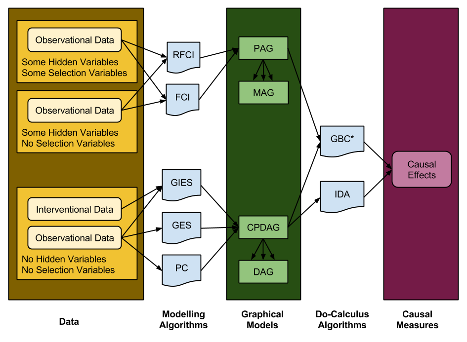
The causal inference process can thus be modeled as three causal artifacts (data, models, measures), and two algorithm categories (modelling, do-calculus).

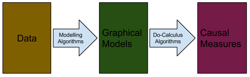
Causal Artifacts

Subtleties With Data

By data we normally mean observational data, which consists of random variables that are independent and identically distributed (iid assumption). However, sometimes our algorithms must process interventional data. What is the difference?

We often have to deal with interventional data in causal inference. In cell biology for example, data is often measured in different mutants, or collected from gene knockdown experiments, or simply measured under different experimental conditions. An intervention, denoted by Pearl’s do-calculus, changes the joint probability distribution of the system; therefore, data samples collected from different intervention experiments are not identically distributed (although still independent).

How do we get from raw data to causal relationships? The secret lies in conditional independence: “Can I use this variable to predict that one, given that I know the value of this third data point?”. Specifically, conditional independence is used to infer a property known as d-separation. D-separation enables us to prune away edges that represent spurious correlations.

We only deal with distributions whose list of conditional independencies perfectly matches the list of d-separation relations of some DAG; such distributions are called faithful. It has been shown that the set of distributions that are faithful is the overwhelming majority [7], so that the assumption does not seem to be very strict in practice.

How do we learn conditional independencies? From an conditional-independence oracle, a black box that unfailingly gives us the correct answers. While such a thing is not realized in the real world, an approximation of it is, in fact, leveraged by our causal algorithms:

In practice, the conditional independence oracle is replaced by a statistical test for conditional independence. For… the PC algorithm, [this replacement] is computationally feasible and consistent even for very high-dimensional sparse DAGs.

But hold on, you may say, data does not just drop into our lap. Data in the real world is incomplete, there may be variables we simply are not tracking (hidden variables). Worse, the subset of data that materializes in front of us is often non-random, but the product of observer bias: selection variables are at work behind the scenes. As you will see, we can and we will account for these.

A Hierarchy Of Graphical Models

I will present four different types of graphical models.

A DAG (directed acyclic graph) is our language of causality. There exist only one type of edge in a DAG:

1. Blank-Arrow. These two edgemarks together represent the direction of causation.

Let’s break down the meaning of the acronym. A DAG is:

• directed due to its arrows
• acyclic in virtue of the fact that you can’t follow the arrows around in a circle.
• graphical because it has nodes and edges

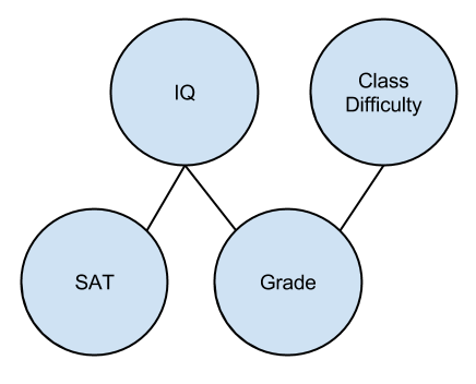
An example:

Notice that this diagram makes the distinction between causality and causation quite clear. SAT may be highly correlated with grade, but it has no causal effect on it. In contrast, Class Difficulty is highly correlated with Grade, and it has a causal effect on it. We tell the difference by d-separation.

Two requisite concepts before we go further.

1. A skeleton is basically a graph with its edgemarks removed.
2. An equivalence class is a set of graphs with the same skeleton but with different edgemarks. They are the set of all possible graphs consistent with the data.

Here’s a skeleton of our DAG:

A CPDAG (completed partially directed acyclic graph) [1] is an equivalence class of DAGs. There exists two types of edges in a CPDAG:

1. Blank-Arrow. The causal direction is displayed clearly if all members of the equivalence class agree.
2. Arrow-Arrow. The causal direction is ambiguous if there is internal disagreement between members of the equivalence class.

An example:

From the above two observations, we see that all DAGs in this equivalence class agree on the V6-V7 relation, but disagree about the V1-V2 relation.

Why would we even need to even conceive of such a graph, if DAGs are enough to represent the state of the world? Because, typically, our algorithms can only produce CPDAGs:

Finding a unique DAG from an independence oracle is in general impossible. Therefore, one only reports on the equivalence class of DAGs in which the true DAG must lie. The equivalence class is visualized using a CPDAG.

But even CPDAGs cannot accommodate those pesky hidden and selection variables!

Suppose, we have a DAG including observed, latent and selection variables and we would like to visualize the conditional independencies among the observed variables only. We could marginalize out all latent variables and condition on all selection variables. It turns out that the resulting list of conditional independencies can in general not be represented by a DAG, since DAGs are not closed under marginalization or conditioning. A class of graphical independence models that is closed under marginalization and conditioning and that contains all DAG models is the class of ancestral graphs.

A MAG (maximal ancestry graph) [8] thus affords for hidden and selection variables. There exist three types of edges in a MAG:

1. Blank-Arrow. Roughly, these edges come from observed variables.
2. Arrow-Arrow. Roughly, these edges come from hidden variables.
3. Blank-Blank. Roughly, these edges come from selection variables.

Let me note in passing that MAGs rely on m-separation, a generalization of d-separation.

The same [motivation for CPDAGs holds] for MAGs: Finding a unique MAG from an independence oracle is in general impossible. One only reports on the equivalence class in which the true MAG lies (a PAG).

A PAG (partial ancestry graph) [11] is an equivalence class of MAGs. There exist six kinds of edges in a PAG:

1. Circle-Circle
2. Circle-Blank
3. Circle-Arrow
4. Blank-Arrow
5. Arrow-Arrow
6. Blank-Blank

PAG edgemarks have the following interpretation:

• Blank: this blank is present in all MAGs in the equivalence class.
• Arrow: this arrow is present in all MAGs in the equivalence class.
• Circle: there is at least one MAG in the equivalence class where the edgemark is a Blank, and at least one where the edgemark is an Arrow.

Causal Measures

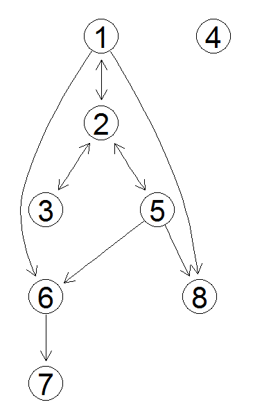
Okay, let’s rewind. Suppose we are in possession of the following CPDAG (whose equivalence class consists of two DAGs):

This diagram allows us to, at a glance, evaluate the relationships between variables. However, it does not address the following question: how strong are the causal relationships? Suppose we wish to quantify the causal strength V1 has over V4, V5, and V6. It turns out that this can be done with the application of Pearl’s methods (including do-calculus). With these techniques in hand, we feed this CPDAG to our do-calculus algorithm, and receive the answer!

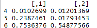
I’ll let the authors explain what this matrix means:

Each row in the output shows the estimated set of possible causal effects on the target variable indicated by the row names. The true values for the causal effect are 0, 0.0, and 0.52 for variables V4, V5 and V6, respectively. The first row, corresponding to variable V4, quite accurately indicates a causal effect that is very close to zero or no effect at all. The second row of the output, corresponding to variable V5, is rather uninformative: although one entry comes close to the true value, the other estimate is close to zero. Thus, we cannot be sure if there is a causal effect at all. The third row is [like V4 in that it is clear].

Causal inference algorithms, therefore, do not completely liberate us from ambiguity: will are still uncertain of the character of the V1-V5 relation.  But, in the V1-V4 and V1-V6 links, we see a different kind of theme: equivalence-class consensus.

Algorithm Categories

Inference Algorithms

• The PC (Peter-Clark) algorithm [10] takes observational, complete data and outputs a CPDAG.
• The GES (Greedy Equivalence Search) algorithm [2] performs the same function, but is faster in virtue of its greediness.
• The GIES (Greedy Interventional Equivalence Search) algorithm [4] generalizes the GES to accommodate interventional data.
• The FCI (Fast Causal Inference) algorithm [9] [10] accepts observational data with an arbitrary number of hidden or selection variables, and produces a PAG.
• The RFCI (Really Fast Causal Inference) algorithm [3] does approximately the same thing, faster!

Do-Calculus Algorithms

• The IDA (Intervention calculus when DAG is Absent) algorithm [5] accepts CPDAGs, and produces a causal measure.
• The GBC (Generalized Backdoor Criterion) algorithm [6] is able to handle hidden variables, but cannot handle selection variables. It takes PAG, MAG, CPDAG, or DAG models and checks whether a causal measure can be estimated. If it can, it goes ahead and gathers precisely that information.

In passing, the authors note that, in [5], “IDA was validated on a large-scale biological system”.

Conclusion

The Causal Landscape

Time to tie everything together!

The State Of The Art

This field is expanding very rapidly. I had the opportunity to read an earlier version of this paper in 2012. To give you a taste of the rate of change, it appears to me that the authors have both produced the mathematics for the GIES and GBC algorithm, and implemented them in R, during the intervening months.

It is useful to gauge a field’s progress in terms of theory constraint – what can we say No to, with these new methods?

• We can say No to non-quantitative rhetoric.
• We can say No to appeals to unconstrained ambiguity.
• We can say No to erroneous causal skeletons.
• We can say No to denials of equivalence-class consensus.

I have a dream that policy makers will pull up CPDAGs of, say, national economics, and use the mathematics to quantitatively identify points-of-agreement. I have a dream that the strengths of our Nos will clear away the smoke from our rhetorical battlefields long enough to find a Yes.

It is such an exciting time to be alive.

References

[1] Andersson et al (1997). “A characterization of Markov equivalence classes for acyclic digraphs”.
[2] Chickering (2002). “Optimal structure identification with greedy search”
[3] Colombo et al. (2012). “Learning High-Dimensional directed acyclic graphs with latent and selection variables”.
[4] Hauser and Buhlmann (2012). “Characterization and greedy learning of interventional Markov equivalence classes of directed acyclic graphs.”
[5] Maathius et al (2010). “Predicting Causal Effects in Large-Scale Systems from Observational Data”.
[6] Maathuis and Colombo (2013). “A generalized backdoor criterion”.
[7] Meek (1995). “Strong completeness and Faithfulness in Bayesian Networks.”
[8] Richardson and Spirtes (2002). “Ancestral Graph Markov Models”
[9] Spirtes et al (1999). “An Algorithm for Causal Inference in the Presence of Latent Variables and Selection Bias.”
[10] Spirtes et al (2000). Causation, Prediction, and Search. Adaptive Computation and Machine Learning, second edition. MIT Press, Cambridge.
[11] Zhang (2008) “On the completeness of orientation rules for causal discovery in the presence of latent confounder and selection bias”.

Appendix: Example Commands

> install.packages(“pcalg”)
> source(“http://bioconductor.org/biocLite.R”)
> biocLite(“RBGL”)
> biocLite(“Rgraphviz”)
> library(“pcalg”)
> data(“gmG”)
> suffStat pc.gmG stopifnot(require(Rgraphviz))
> par(mfrow = c(1,2))
> plot(gmG$g, main = “”) ; plot (pc.gmG, main = “”)
> idaFast(1, c(4,5,6), cov(gmG$x), pc.gmG@graph)