Part Of: [Advanced Inference In Graphical Models] sequence

Table Of Contents

• Cliquish Nodes
• The Mechanics Of Variable Elimination
• A Question Of Order
• Enter Graphical Models
• Murderous Cliques
• Takeaways

Cliquish Nodes

Fully-connected networks have some interesting properties. Let’s create a vocabulary to reason about them in more nuanced graphs.

• Let clique be a subset of nodes in a graph that are fully connected. Call the set of all cliques C.
• Let maximal clique be a clique that cannot remain a clique by including any one more adjacent vertex.
• Let maximum clique be a clique C_mm for which |C_mm| =  max(|C_x|) for each C_x in C.

An example may help, you say?!

Our three sets in action:

• Cliques: {{1}, {2}, {3}, {4}, {5}, {1, 2}, {2, 3}, {1, 3}, {2, 4}, {3, 4}, {2, 5}, {1, 2, 3}, { 2, 3, 4 }}
• Maximal Cliques: {{1, 2, 3}, {2, 3, 4}, {2, 5}}
• Maximum Cliques: {{1, 2, 3}, {2, 3, 4}}

The Mechanics Of Variable Elimination

The basic point of variable elimination is to push summation signs as far to the right as possible, to reduce computational complexity (you no longer have to ask factors not involving x_i, to sum over it).

Let us call this the factor grouping step:

See how we pulled x_i summation to the right?

Once we have a single summation over only the relevant factors, we proceed. The resultant aggregation will no longer contain X_i; therefore, let us call this operation variable elimination step.

To be clear, the above notation is a psi_{1, 2} – but the one is scratched out, to represent its elimination.

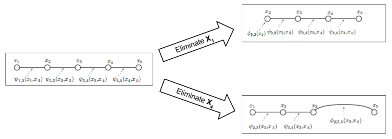
Putting these two steps together, we can now understand the process of eliminate a variable from our model. Consider the task of eliminating x₁ from the following model:

The above image captures the process for eliminating one variable. To find p(x₃, x₄), we must eliminate two more. Imagine we choose X₅ to eliminate next, and then X₂.  The resulting equation will bear our answer, the value of p(x₃, x₄).

A Question Of Order

In the above example, we chose the following variable elimination ordering: (1, 5, 2). But other orderings are possible. How does (1, 5, 2) compare to (2, 1, 5) or (5, 2, 1)?

How might we rank the desirability of different variable elimination orderings? An attractive metric is computational complexity: we should choose the ordering that minimizes the amount of required CPU muscle.

Enter Graphical Models

Graphical models provides us a way to visually inspect what used to be solely manipulations of formulae. Here is the exact same computation as above, but with pictures:

The key insight: the reconstituted graphical model (GM) is equivalent to the original GM.

HOWEVER! Such equivalence is not guaranteed! Consider what happens when we eliminate X₄ first:

Notice how the reconstituted GM diverges from the original GM: a new edge has been added between x3 and x5. Let us call this a fill-in edge.

Fill-in edges are bad news. The edges of the original graph constitute its family: when you add edges, the boundaries of the family expands, which hurts inference processes. Recasting our lens to asymptotic analysis, fill-in edges represent an added computational burden – tables whose dimensionality we would rather not compute over.

Why does choosing to first eliminate X₄ create a fill-in edge? To understand these, we’ll need to apply deep mathematics to analyze relationships between different families F(G, R).

Murderous Cliques

Let us use MRF-clique semantic interchangeability to look at fill-in edges with the lens of clique semantics. Consider again the fill-in edge phenomenon encountered above:

In the original graph (left), the maximal cliques are {{1, 2}, {2, 3}, {3, 4}, {4, 5}}. The key insight is as follows:

• Existence of f₁(x_A, x_B) suggests that G[A ∪ B] should be a clique, and existence of f₂(x_B, x_C) suggests G[B ∪ C] should be a clique.
• After summation, existence of f(x_A, x_C) suggests that G[A ∪ C] should also be a clique (if it is not already).

In other words:

• After v is eliminated, all of its former neighbors must form a clique. If they do not, undesirable fill-in edges will be added to our graph, and the family will expand.

We can explain the x₄ fill-in edge because its neighbors (x₃ and x₅) were not already a clique.

Thus, variable elimination ordering becomes a question of analyzing the cliques of a graph. Let us call this perspective murderous cliques for short! 🙂

Takeaways

• Cliques are graph subsets that are fully connected.
• Variable elimination is a computational process that first bundles like factors together, and then eliminates a variable via “summing it out”.
• The order in which one eliminates irrelevant variables is computationally significant.
• Sometimes, variable elimination creates undesirable fill-in edges – edges that breach the family contract & expands the boundaries of the graphical model.
• Deep parallels exist between clique semantics and traditional MRF factoralization.
• Fill-in edges happen because the former neighbors of a fill-in edge must form a clique.
• In conclusion, when selecting the order in which to eliminate variables, if possible, choose the variable whose neighbors already form a clique.