Lie Detection: Gullible By Default

Part Of: Language sequence
Content Summary: 1300 words, 13 min read
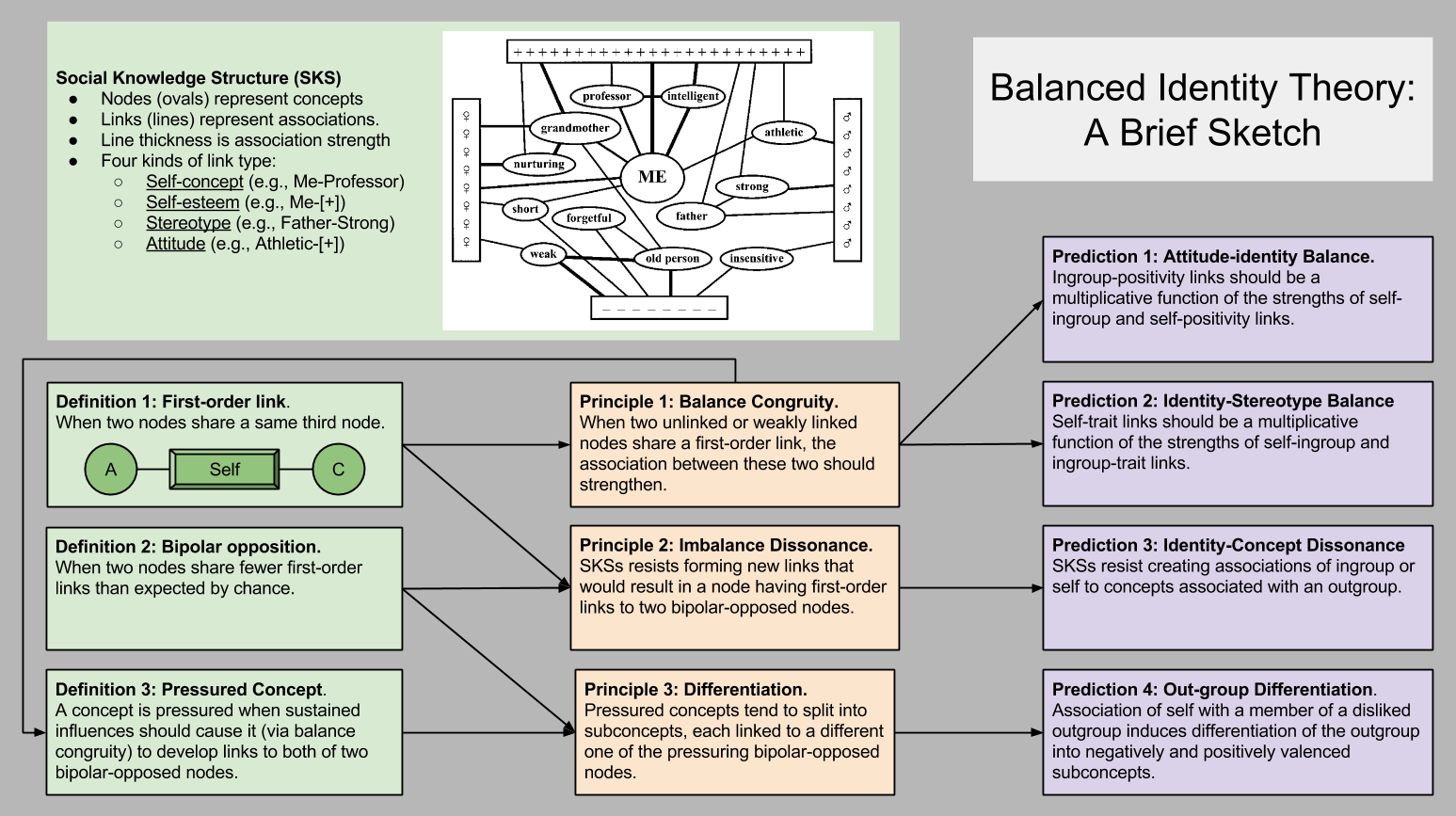
Two Tagging Methods

Imagine a library of a few million volumes, a small number of which are fiction. There are at least two reasonable methods with which one could distinguish fiction from nonfiction at a glance:

  1. Paste a red tag on each volume of fiction and a blue tag on each volume of nonfiction.
  2. Tag the fiction and leave the nonfiction untagged.

Perhaps the most striking feature of these two different systems is how similar they are. Despite the fact that the two libraries use somewhat different tagging systems, both ultimately accomplish the same end. Imagine each book If the labeling was done by a machine inside of a tiny closet – if a library user could not see with her own eyes the method employed, is there any hope of her discovering the truth method employed?

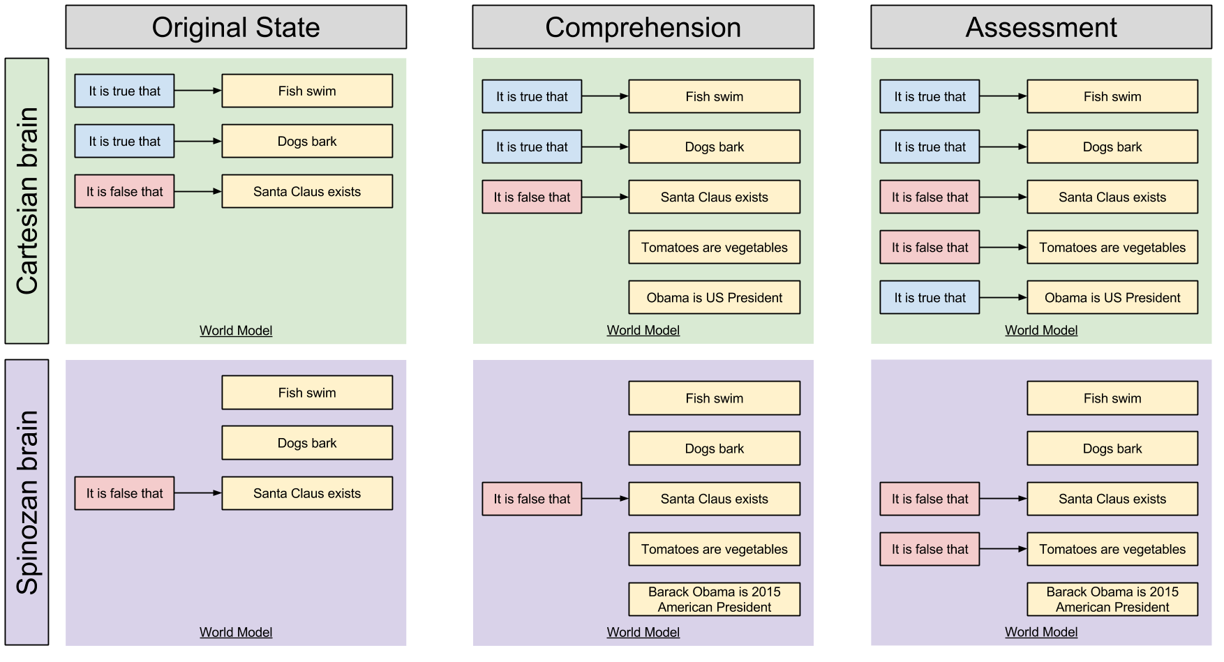
This is exactly the problem faced by cognitive scientists trying to understand the nature of belief. Your brain is responsible for maintaining a collection of beliefs (the mental library). Some of these beliefs are marked true (e.g., “fish swim”); others are marked false (e.g., “Santa Claus is real”). As philosophers in the 18th century discovered, your brain could process truth from falsehood in two distinct ways:

  1. Rene Descartes thought the brain uses the red-blue system. That is, it first tries to comprehend an idea (import the book) and then evaluate its status (give it the appropriate color).
  2. Baruch Spinoza thought the brain uses the tagged-untagged system. That is, it first tries to comprehend an idea (import the book) and then check whether it is fiction (decide whether it needs to be tagged).

Here is a graphical representations of the two brains:

Default Gullibility- Two World Model Updating Systems

Would The Real Brain Please Stand Up?

Ideal mental systems have unlimited processing resources and an unstoppable tagging system. Real mental systems operate under imperfect conditions and a finite pool of resources, which causes these mental processes to sometimes fail. Sometimes, your brain isn’t able to assess beliefs at all.

What happens when a Cartesian red-blue brain is unable to fully assess incoming beliefs? Well, if the world model is left alone after comprehension (middle column), then resultant beliefs are neither marked true nor false, easily distinguishable from more trustworthy beliefs.

What happens when a Spinozan tagged-untagged brain cannot assess an incoming belief? Well, if its World Model processing stops after comprehension (middle column), then the novel claims appear identical to true beliefs.

On the Cartesian system, comprehension is distinct from acceptance. On a Spinozan system, comprehension is acceptance, and an additional (optional!) effort is required to unaccept belief. Cartesian brains are innately analytic, Spinozan brains are innately gullible.

So which is it? Is your brain Cartesian or Spinozan?

Three Reasons Why Your Brain Is Spinozan

Three streams of evidence independently corroborate the existence of the Spinozan brain.

First, scientists have confirmed time and again that distraction amplifies gullibility.

[Festinger & Maccoby 1964] demonstrated that subjects who listened to an untrue communication while attending to an irrelevant stimulus were particularly likely to accept the propositions they comprehended (see [Baron & Miller 1973] for a review of such studies)

When resource-depleted persons are exposed to doubtful propositions (i.e., propositions that they normally would disbelieve), their ability to reject those propositions is markedly reduced (see [Petty & Cacioppo 1986] for a review).

This effect appears in more complex scenarios, too. Suppose your friend Clyde says that “dragons exist”. In this scenario, the brain may not simply wish to reject that (first-order) claim, but also implement lie detection via rejecting the second-order proposition that “Clyde thinks that dragons exist”.

Default Gullibility- Two Types Of Negation (1)

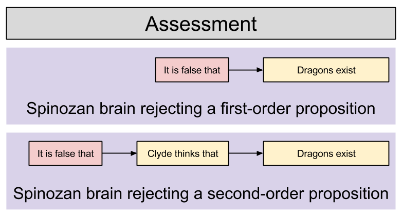
In the context of second-order propositions, distraction causes an even stronger inability to reject claims:

After decades of research activity, both the lie-detection and attribution literatures have independently concluded that people are particularly prone to accept the second-order propositions implicit in others’ words and deeds (for reviews of these literatures see, respectively, [Zuckerman, Depaulo, & Rosenthal 1981] and [Jones 1979]. What makes this phenomenon so intriguing is that people accept these assertions even when they know full well that the assertions stand an excellent chance of being wrong. For example, if an authority asks someone to read aloud a prepared statement (e.g., “I am in favor of federal protection of armadillos”), people [still] assume that the speaker believes the words coming out of the speaker’s mouth. This robust tendency is precisely the sort that a resource-depleted Spinozan system should display.

Not only does dubious position assertions more believable amidst distraction, the opposite of reasonable denials are also likely to be affirmed. That is, resource depletion will cause statements like “Bob Talbert not linked to Mafia” to induce belief in “Bob Talbert linked to Mafia”. The Cartesian model predicts no such asymmetry in response to resource depletion during assessment.

Second, children develop the ability to believe long before the ability to disbelieve.

The ability to deny propositions is, in fact, one of the last linguistic abilities to emerge in childhood [Bloom 1970] [Pea 1980] Although very young children may use the word no to reject, the denial function of the word is not mastered until quite a bit later.

Furthermore, young children are particularly prone to accept propositions uncritically (see [Ceci et al 1987]). Although such hypersuggestibility is surely exacerbated by the child’s inexperience and powerlessness, young children are more suggestible than older children even when such factors are taken into account [Ceci et al 1987].

Third, linguistic evidence shows that negative beliefs take longer to assess, and appear less frequently in practice.

A fundamental assumption of psycholinguistic research is that “complexity of in thought tends to be reflected in complexity of expression”, and vice versa. The markedness of a word is usually considered the clearest index of linguistic complexity… The Spinozan hypothesis states that acceptance is a more complex operation than is acceptance and, interestingly enough, the English words that indicate acceptance of ideas are generally unmarked. That is, our everyday language has us speaking of propositions as acceptable and unacceptable instead of rejectable and unrejectable. Indeed, people even speak of belief and disbelief more naturally than they speak of doubt and undoubt.

People are generally quicker to assess true statements, than false statements [Gough 1965].

How Should We Then Think?

Frankly, this was a difficult article to post. Knowing about biases can hurt people; that is, learning about their own flaws can make people defensive and inflexible.

But this sobering post need not cause us to abandon curiosity and pursuit of truth. It is the mark of an educated mind embrace a thought without flinching, to explore its consequences without fear. It is possible to change your mind.

Takeaways

This article was inspired by [Gilbert 1991] How Mental Systems Believe. Points to remember:

  • How to tell truth from falsehood? You can either tag all beliefs true or false (Cartesian system) or only tag false belief (Spinozan system)
  • Beliefs aren’t always fully analyzed. But in a Spinozan system, unassessed beliefs appear true – the system is credulous by default.
  • Comprehension is belief: gullibility is innate. Only critical thinking is optional, effortful, and prone to failure. Your brain is Spinozan.
    • How do we know? Because distraction causes thinkers to become more gullible
    • How do we know? Because young children are very suggestible, only later acquiring the ability to be skeptical
    • How do we know? Because negative beliefs take longer to assess, have more complex words, and appear less frequently in practice.
  • The great master fallacy of the human mind is believing too much.

References

  • [Baron & Miller 1973] The relation between distraction and persuasion.
  • [Bloom 1970] Language development: Form and function in emerging grammars.
  • [Ceci et al 1987] Suggestibility of children’s memory: Psychological implications.
  • [Festinger & Maccoby 1964] On resistance to persuasive communications.
  • [Gough 1965] The verification of sentences: The effects of delay of evidence and sentence length.
  • [Jones 1979] The rocky road from acts to dispositions.
  • [Pea 1980] The development of negation in early child language.
  • [Petty & Cacioppo 1986] The elaboration likelihood model of persuasion.
  • [Zuckerman, Depaulo, & Rosenthal 1981] Verbal and nonverbal communication of deception.
Advertisement

The Causal Inverse Problem

Part Of: Causal Inference sequence
Content Summary: 1000 words, 10 min read.

A Riddle

We begin with a riddle!

riddle

We will arrive at an answer by the end of this article. 🙂  Our journey will begin with a survey of a field within visual processing.

The Mystery Of Stereopsis

Stereopsis is the computational construction of depth from visual data. Physics is embedded in three spatial dimensions, yet your retinae are essentially 2D (imagine wrapping a sheet of paper around half of a sphere). Depth information can be gleaned from comparing the disparities between two similar images, and applying geometric principles to compute depth.  The dual images do not have to come from two eyes, either!  Close one eye, and the brain can still infer depth from motion (by comparing two images from the same eye across time).

However, stereopsis is plagued by the problem of underdetermination. The following diagram motivates this nicely:

depth_matrix

The inverse projection is your mental model of the environment. However, your brain only possesses 2D retinal images.  To recreate the environment, we consider image matches:

  1. Gray hexes are matches (left image color does not match right color)
  2. White hexes are non-matches.

The grey hexes are possible 3D interpretations of the 2D images. The black hexes are correct 3D interpretation. The brain must select a subset of grey hexes to be black hexes (which possible interpretation is veridical). This is the visual inverse problem.

The Secret To Depth Reconstruction

Visual data alone provides no obvious solution to the visual inverse problem. How then do we explain interpretation consensus (that mammals almost always agree on one particular depth-interpretation), and interpretation veracity (that the consensus is almost always correct)?

Consider the inverse projection again. Do you notice that the black hexes (correct answers) tend to be side-by-side?

In general, we might prefer interpretations (grey hexes) that are spatially continuous. The brain in fact uses cues like spatial continuity to solve the visual inverse problem.

Spatial continuity helps us begin to understand interpretation consensus. But it alone is insufficient for selecting only one possible interpretations. The brain relies on a total of six cognitive assumptions:

  1. Existence Of Surfaces: The visible world can be regarded as being composed of smooth surfaces having reflectance functions whose spatial structure may be elaborate.
  2. Hierarchical Organization: A surface’s reflectance function is often generated by a number of different processes, each operating at a different scale.
  3. Similarity: The items generated on a given surface by a reflectance-generating process acting at a given scale tend to be more similar to one another in their size, local contrast, color, and spatial organization that to other items on that surface.
  4. Spatial Continuity: Markings generated on a surface by a single process are often spatially organized – they are arranged in curves or lines and possibly create more complex patterns.
  5. Continuity Of Discontinuities: The loci of discontinuities in depth or in surface orientation are smooth almost everywhere.
  6. Continuity Of Flow: If direction of motion is ever discontinuous at more than one point – along a line, for example – then an object boundary is present.

In his book, Marr shows how these assumptions can be expressed in computational algorithms that solve the visual inverse problem. Further, neurobiological evidence suggests that one of them is the actual mechanism used by our brains.

The Nature Of Cognitive Assumptions

Why do these cognitive assumptions work? Because Earth’s photic environment features important statistical regularities. We assume similarity because most within-object visual characteristics tends to be more homogenous than that between objects.

These six assumptions also explain many optical illusion phenomena. Most optical illusions represent statistical deviations that violate our reliance on the above assumptions. For example, the depth illusion at the beginning of the article violates our our brain’s natural intuitions about perspective. Such illusions therefore are not a misfiring of an individual human vision system. It is a design consequence.

How do our brains know about these statistical regularities? Two vehicles suggest themselves:

  1. Natural Selection. Since the world is rife with statistical regularities, organisms that encode this structure more efficiently will tend to outperform their peers.
  2. Developmental Learning. In addition to short-term episodes visual inference, the visual system might itself learn to retain information about statistical regularities. This is e.g., suggested in recent research on visual normalization.

If physics were different, the statistics of everyday vision would be different, and thus a different collection of cognitive assumptions would have emerged.

Crossing The Bridge To Causal Inference

Gopnik et al suggest that cognitive assumptions are not unique to vision. Causal inference also relies on statistical regularities of causations. Specifically, the following causal assumptions are relied on by the brain:

  1. Markov Assumption. If the conditional probability distribution of future states of the process (conditional on both past and present values) depends only upon the present state; that is, given the present, the future does not depend on the past.
  2. Faithfulness Assumption. In the joint distribution on the variables in the graph, all conditional independencies are consequences of the Markov assumption applied to the graph.

The Markov assumption says that there will be certain conditional independencies if the graph has a particular structure, the faithfulness assumption says that there will be those conditional independencies only if the graph has a particular structure. The faithfulness assumption supplies the other half of the biconditional.

Solving The Riddle

Statisticians have long known about Simpson’s Paradox: “a paradox in which a trend that appears in different groups of data disappears when these groups are combined, and the reverse trend appears for the aggregate data”.

Image 2 summarizes this effect well: only when you disaggregate gender can you see the deleterious effect of the drug on recovery probability.

riddle

These two figures are similar in virtue of the fact that they violate cognitive assumptions embedded in all neurotypical adults:

  • Image 1 violate visual assumptions (perspective assumptions)
  • Image 2 violate causal assumptions (faithfulness assumption)

References

  • Marr (1982). Vision.
  • Gopnik et al (2004). A Theory of Causal Learning in Children: Causal Maps and Bayes Nets

Causal Inference with pcalg

Part Of: Causal Inference sequence
Content Summary: 2200 words, 22 min read

Introduction

In this post, we’re going to explore one way to do causal inference, as described in the following article:

Title: More Causal Inference with Graphical Models in R Package pcalg
Authors: Kalisch, K et. al
Published: 2014
Citations: 49 (note: as of 04/2014)
Link: Here (note: not a permalink)

Setting The Stage

Statistics is haunted by soundbites like few other professions. “Lies, damned lies, and statistics” needs to die. The way to mitigate deceit is not ignorance, it is the promotion of statistical literacy. “Correlation does not imply causation” should also be expunged. There must be a way to affirm the significance of spurious correlations without blinding people to the fact that causation can be learned from correlation.

When you read someone like C.S. Peirce, you will hear claims that causality is dead. Causality is, indeed, a very ancient topic. In the medieval period, the Aristotelian story about causality – a quadpartite distinction of Material Cause, Formal Cause, Efficient Cause, Final Cause – dominated the intellectual landscape. The moderns, however, were largely dissatisfied with this story; with the Newtonian introduction of forces, the above distinction began to fade into the background. So why are scientists now trying to reclaim causality from the annals of philosophy?

Enter Judea Pearl, champion of Bayesian networks and belief propagation. Dissatisfied with his near-godlike contributions to humanity, he proceeded to found modern causal theory with this text, appropriately named Causality. The reason that causality has reclaimed its sexiness is because Pearl found a way to quantize it, to update one’s beliefs about it, from raw data. Pearl grounds his version of causality in counterfactual reasoning, and borrows heavily from modal logic (c.f., possible worlds). He also introduces the notion of do-calculus, noting that there needs to exist within probability theory, operators that model action (just as “|” models observation). This SEP section explores the philosophical underpinnings of the theory in more depth.

Pearl’s movement is picking up speed. Today, you’ll find causal inference journals, conferences bent on exploring the state of the art, and business leaders trying to harness its powers to make a profit. Causal inference will be the next wave of the big data movement. It explains how human brains create concepts. It is the future of politics.

Put on your seatbelts. We’re going to take causal inference software – an R package named pcalg – out for a drive. If you want the driver’s wheel, you can have it: install RStudio, and refer to the step-by-step tutorial in the paper (or, see Appendix below). This article won’t attempt to install a complete understanding of causal models; I am content to build up your vocabulary.

The causal inference process can thus be modeled as three causal artifacts (data, models, measures), and two algorithm categories (modelling, do-calculus).

Causal Models- Overview

Causal Artifacts

Subtleties With Data

By data we normally mean observational data, which consists of random variables that are independent and identically distributed (iid assumption). However, sometimes our algorithms must process interventional data. What is the difference?

We often have to deal with interventional data in causal inference. In cell biology for example, data is often measured in different mutants, or collected from gene knockdown experiments, or simply measured under different experimental conditions. An intervention, denoted by Pearl’s do-calculus, changes the joint probability distribution of the system; therefore, data samples collected from different intervention experiments are not identically distributed (although still independent).

How do we get from raw data to causal relationships? The secret lies in conditional independence: “Can I use this variable to predict that one, given that I know the value of this third data point?”. Specifically, conditional independence is used to infer a property known as d-separation. D-separation enables us to prune away edges that represent spurious correlations.

We only deal with distributions whose list of conditional independencies perfectly matches the list of d-separation relations of some DAG; such distributions are called faithful. It has been shown that the set of distributions that are faithful is the overwhelming majority [7], so that the assumption does not seem to be very strict in practice.

How do we learn conditional independencies? From an conditional-independence oracle, a black box that unfailingly gives us the correct answers. While such a thing is not realized in the real world, an approximation of it is, in fact, leveraged by our causal algorithms:

In practice, the conditional independence oracle is replaced by a statistical test for conditional independence. For… the PC algorithm, [this replacement] is computationally feasible and consistent even for very high-dimensional sparse DAGs.

But hold on, you may say, data does not just drop into our lap. Data in the real world is incomplete, there may be variables we simply are not tracking (hidden variables). Worse, the subset of data that materializes in front of us is often non-random, but the product of observer bias: selection variables are at work behind the scenes. As you will see, we can and we will account for these.

A Hierarchy Of Graphical Models

I will present four different types of graphical models.

A DAG (directed acyclic graph) is our language of causality. There exist only one type of edge in a DAG:

  1. Blank-Arrow. These two edgemarks together represent the direction of causation.

Let’s break down the meaning of the acronym. A DAG is:

  • directed due to its arrows
  • acyclic in virtue of the fact that you can’t follow the arrows around in a circle.
  • graphical because it has nodes and edges

An example:

Causal Models- DAG

Notice that this diagram makes the distinction between causality and causation quite clear. SAT may be highly correlated with grade, but it has no causal effect on it. In contrast, Class Difficulty is highly correlated with Grade, and it has a causal effect on it. We tell the difference by d-separation.

Two requisite concepts before we go further.

  1. A skeleton is basically a graph with its edgemarks removed.
  2. An equivalence class is a set of graphs with the same skeleton but with different edgemarks. They are the set of all possible graphs consistent with the data.

Here’s a skeleton of our DAG:

Causal Models- DAG Skeleton

A CPDAG (completed partially directed acyclic graph) [1] is an equivalence class of DAGs. There exists two types of edges in a CPDAG:

  1. Blank-Arrow. The causal direction is displayed clearly if all members of the equivalence class agree.
  2. Arrow-Arrow. The causal direction is ambiguous if there is internal disagreement between members of the equivalence class.

An example:

cpdag

From the above two observations, we see that all DAGs in this equivalence class agree on the V6-V7 relation, but disagree about the V1-V2 relation.

Why would we even need to even conceive of such a graph, if DAGs are enough to represent the state of the world? Because, typically, our algorithms can only produce CPDAGs:

Finding a unique DAG from an independence oracle is in general impossible. Therefore, one only reports on the equivalence class of DAGs in which the true DAG must lie. The equivalence class is visualized using a CPDAG.

But even CPDAGs cannot accommodate those pesky hidden and selection variables!

Suppose, we have a DAG including observed, latent and selection variables and we would like to visualize the conditional independencies among the observed variables only. We could marginalize out all latent variables and condition on all selection variables. It turns out that the resulting list of conditional independencies can in general not be represented by a DAG, since DAGs are not closed under marginalization or conditioning. A class of graphical independence models that is closed under marginalization and conditioning and that contains all DAG models is the class of ancestral graphs.

A MAG (maximal ancestry graph) [8] thus affords for hidden and selection variables. There exist three types of edges in a MAG:

  1. Blank-Arrow. Roughly, these edges come from observed variables.
  2. Arrow-Arrow. Roughly, these edges come from hidden variables.
  3. Blank-Blank. Roughly, these edges come from selection variables.

Let me note in passing that MAGs rely on m-separation, a generalization of d-separation.

The same [motivation for CPDAGs holds] for MAGs: Finding a unique MAG from an independence oracle is in general impossible. One only reports on the equivalence class in which the true MAG lies (a PAG).

A PAG (partial ancestry graph) [11] is an equivalence class of MAGs. There exist six kinds of edges in a PAG:

  1. Circle-Circle
  2. Circle-Blank
  3. Circle-Arrow
  4. Blank-Arrow
  5. Arrow-Arrow
  6. Blank-Blank

PAG edgemarks have the following interpretation:

  • Blank: this blank is present in all MAGs in the equivalence class.
  • Arrow: this arrow is present in all MAGs in the equivalence class.
  • Circle: there is at least one MAG in the equivalence class where the edgemark is a Blank, and at least one where the edgemark is an Arrow.

Causal Measures

Okay, let’s rewind. Suppose we are in possession of the following CPDAG (whose equivalence class consists of two DAGs):

cpdag

This diagram allows us to, at a glance, evaluate the relationships between variables. However, it does not address the following question: how strong are the causal relationships? Suppose we wish to quantify the causal strength V1 has over V4, V5, and V6. It turns out that this can be done with the application of Pearl’s methods (including do-calculus). With these techniques in hand, we feed this CPDAG to our do-calculus algorithm, and receive the answer!

effects

I’ll let the authors explain what this matrix means:

Each row in the output shows the estimated set of possible causal effects on the target variable indicated by the row names. The true values for the causal effect are 0, 0.0, and 0.52 for variables V4, V5 and V6, respectively. The first row, corresponding to variable V4, quite accurately indicates a causal effect that is very close to zero or no effect at all. The second row of the output, corresponding to variable V5, is rather uninformative: although one entry comes close to the true value, the other estimate is close to zero. Thus, we cannot be sure if there is a causal effect at all. The third row is [like V4 in that it is clear].

Causal inference algorithms, therefore, do not completely liberate us from ambiguity: will are still uncertain of the character of the V1-V5 relation.  But, in the V1-V4 and V1-V6 links, we see a different kind of theme: equivalence-class consensus.

Algorithm Categories

Inference Algorithms

  • The PC (Peter-Clark) algorithm [10] takes observational, complete data and outputs a CPDAG.
  • The GES (Greedy Equivalence Search) algorithm [2] performs the same function, but is faster in virtue of its greediness.
  • The GIES (Greedy Interventional Equivalence Search) algorithm [4] generalizes the GES to accommodate interventional data.
  • The FCI (Fast Causal Inference) algorithm [9] [10] accepts observational data with an arbitrary number of hidden or selection variables, and produces a PAG.
  • The RFCI (Really Fast Causal Inference) algorithm [3] does approximately the same thing, faster!

Do-Calculus Algorithms

  • The IDA (Intervention calculus when DAG is Absent) algorithm [5] accepts CPDAGs, and produces a causal measure.
  • The GBC (Generalized Backdoor Criterion) algorithm [6] is able to handle hidden variables, but cannot handle selection variables. It takes PAG, MAG, CPDAG, or DAG models and checks whether a causal measure can be estimated. If it can, it goes ahead and gathers precisely that information.

In passing, the authors note that, in [5], “IDA was validated on a large-scale biological system”.

Conclusion

The Causal Landscape

Time to tie everything together!

Causal Models- Landscape

The State Of The Art

This field is expanding very rapidly. I had the opportunity to read an earlier version of this paper in 2012. To give you a taste of the rate of change, it appears to me that the authors have both produced the mathematics for the GIES and GBC algorithm, and implemented them in R, during the intervening months.

It is useful to gauge a field’s progress in terms of theory constraint – what can we say No to, with these new methods?

  • We can say No to non-quantitative rhetoric.
  • We can say No to appeals to unconstrained ambiguity.
  • We can say No to erroneous causal skeletons.
  • We can say No to denials of equivalence-class consensus.

I have a dream that policy makers will pull up CPDAGs of, say, national economics, and use the mathematics to quantitatively identify points-of-agreement. I have a dream that the strengths of our Nos will clear away the smoke from our rhetorical battlefields long enough to find a Yes.

It is such an exciting time to be alive.

References

[1] Andersson et al (1997). “A characterization of Markov equivalence classes for acyclic digraphs”.
[2] Chickering (2002). “Optimal structure identification with greedy search”
[3] Colombo et al. (2012). “Learning High-Dimensional directed acyclic graphs with latent and selection variables”.
[4] Hauser and Buhlmann (2012). “Characterization and greedy learning of interventional Markov equivalence classes of directed acyclic graphs.”
[5] Maathius et al (2010). “Predicting Causal Effects in Large-Scale Systems from Observational Data”.
[6] Maathuis and Colombo (2013). “A generalized backdoor criterion”.
[7] Meek (1995). “Strong completeness and Faithfulness in Bayesian Networks.”
[8] Richardson and Spirtes (2002). “Ancestral Graph Markov Models”
[9] Spirtes et al (1999). “An Algorithm for Causal Inference in the Presence of Latent Variables and Selection Bias.”
[10] Spirtes et al (2000). Causation, Prediction, and Search. Adaptive Computation and Machine Learning, second edition. MIT Press, Cambridge.
[11] Zhang (2008) “On the completeness of orientation rules for causal discovery in the presence of latent confounder and selection bias”.

Appendix: Example Commands

> install.packages(“pcalg”)
> source(“http://bioconductor.org/biocLite.R”)
> biocLite(“RBGL”)
> biocLite(“Rgraphviz”)
> library(“pcalg”)
> data(“gmG”)
> suffStat pc.gmG stopifnot(require(Rgraphviz))
> par(mfrow = c(1,2))
> plot(gmG$g, main = “”) ; plot (pc.gmG, main = “”)
> idaFast(1, c(4,5,6), cov(gmG$x), pc.gmG@graph)

Machery: Précis of Doing without Concepts

Content Summary: 2600 words, 26 minute read.

Introduction

There is no secret that the academic field of concepts is in disarray. In this article, Machery attempts to weave these disparate traditions into a compelling whole.  But first, a quote which serves to motivate what follows:

Why do cognitive scientists want a theory of concepts? Theories of concepts are meant to explain the properties of our cognitive competences. People categorize the way they do, they draw the inductions they do, and so on, because of the properties of the concepts they have. Thus, providing a good theory of concepts could go a long way towards explaining some important higher cognitive competences.

Summarization text is grayscale, my commentary is in orange.

Article Metadata

  • Article: Précis of Doing without Concepts
  • Author: Edouard Machery
  • Published: 11/2009
  • Citations: 178 (note: as of 04/2014)
  • Link: Here (note: not a permalink)

Section 1. Regimenting the use of concept in cognitive science

We start with definitions!

The world is not an undifferentiated sea of chaos. It has statistically noticeable patterns – “joints”. Let us call these delightful patterns in nature a category (or a natural kind). But categories are things in the world, and your mind must somehow learn these categories for itself. Plato once described the act of reasoning as: “That of dividing things again by classes, where the natural joints are, and not trying to break any part, after the manner of a bad carver.” (Phaedrus, 265e). This analogy – to carve nature at its joints – is what concept processes do. Concepts represent categories in your brain.

Let’s get specific about the properties of concepts. Machery defines concept as something that:

  1. Can be about a class, event, substance, or individual.
  2. Nonproprietary, not constrained by the underlying type of represented information.
  3. Constitutive elements can vary over time and across individuals.
  4. Some elements of information about X may not fit into the concept of X; let us call these data background knowledge.
  5. They are used by Default (I will define this in Section 3).

Section 2. Individuating concepts

Is it possible for an individual to possess different concepts of the same category?
Can Kevin possess two concepts of the category of chair?
Yes.
How do we individuate two related pieces of information, that would otherwise fall under the same concept?

I propose [that] when two elements of information about x, A and B, fulfill either of these [individuation] criteria, they belong to distinct concepts:

  • Connection Criterion: If retrieving A (e.g., water is typically transparent) from LTM and using it in a cognitive process (e.g., a categorization process) does not facilitate the retrieval of B (e.g., water is made of molecules of H20) from LTM and its use in some cognitive process, then A and B belong to two distinct concepts (WATER1 and WATER2).
  • Coordination Criterion: If A and B yield conflicting judgments (e.g., the judgment that some liquid is water and the judgment that this very liquid is not water) and if I do not view either judgment as defeasible in light of the other judgment (i.e., if I hold both judgments to be equally authoritative), then A and B belong to two distinct concepts (WATER1 and WATER2).

Section 3. Defending the proposed notion of concept

Time to explore our last property of concepts, “used by Default”. Default is a name for “the assumption that some bodies of knowledge are retrieved by default when one is categorizing, reasoning, drawing analogies, and making inductions”.  Say you are given a word problem involving counting apples and oranges. Default is the claim that a flood of concepts – including but not limited to arithmetic, the apple, the orange, trees, and fruit – will be drawn from long term memory (LTM) stores, and made available to your mental processes automatically.

At least two research traditions go against this claim:

  1. Concepts are not retrieved from LTM automatically, they are rather summoned via conscious attention.
  2. Concepts are drawn from LTM automatically, but they are constructed on-the-fly.  When you see an apple, you do not load a concept of apple that was hashed out long ago, your mind queries your LTM for apple-related background knowledge, constructing transient concepts especially tailored for the peculiarities of the task at hand.

Machery makes three counterpoints:

  1. Only a pronounced amount of recall variability (e.g., highly divergent results for tweaking minor parameters of a word problem) would falsify Default in favor of on-the-fly concept construction.
  2. Empirical investigations only reveal moderate levels of recall variability.
  3. A substantial amount of evidence supports Default.

Section 4. Developing a psychological theory of concepts

A psychological theory of concepts must treat the following concerns:

  • The nature of the information constitutive of concepts
  • The nature of the processes that use concepts
  • The nature of the vehicle of concepts
  • The brain areas that are involved in possessing concepts
  • The processes of concept acquisition

Section 5. Concept in cognitive science and in philosophy

The gist of the section:

Although both philosophers and cognitive scientists use the term concept, they are not talking about the same things. Cognitive scientists are talking about a certain kind of bodies of knowledge, they attempt to explain the properties of our categorization, inductions etc; whereas philosophers are talking about that which allows people to have propositional attitudes. Many controversies between philosophers and psychologists about the nature of concepts are thus vacuous.

An amusing aside that I desire to explicitly ground the definition of vacuous into some theory of concepts, when I come to treat pragmatism.

Anyways, my tentative attempt to restate the above: Philosophers concern themselves with category-concept fidelity, whereas cognitive scientists concern themselves with the lifecycle of the concept within the mental ecosystem.

Section 6. The heterogeneity hypothesis versus the received view

Machery defines the received view as the assumption that, beyond differences within concept subject-matter, concepts share many properties that are scientifically interesting. Machery suggests that this a mistake, and that the evidence suggests the existence of several distinct types of concept. Concept, in other words, is itself not a category (natural kind). A nuanced sentence if you’ve ever heard one. 🙂

The Heterogeneity Hypothesis, in contrast, claims that processes that produce concepts are distinct, that they share little in common.

Section 7. What kind of evidence could support the heterogeneity hypothesis?

Three kinds of evidence are predicted:

  1. When the conceptualization processes fire individually, we expect each to receive strong confirmation in just those experiments.
  2. When the conceptualization processes fire together, outputs may be incongruent, requiring mediation; we thus expect processing delays.
  3. Although the epistemology of dissociations is intricate, we should expect confirmation from neuropsychological data analysis.

Section 8. The fundamental kinds of concepts

Three different kinds of concepts exist in your cognitive architecture:

  1. Prototypes are bodies of statistical knowledge about a category, a substance, a type of event, and so on. For example, a prototype of dogs could store some statistical knowledge about the properties that are typical of dogs and/or the properties that are diagnostic of the class of dogs… Prototype are typically assumed to be used in cognitive processes that compute similarity linearly.
  2. Exemplars are bodies of knowledge about individual members of a category (e.g., Fido, Rover), particular samples of a substance, and particular instances of a kind of event (e.g., my last visit to the dentist). Exemplars are typically assumed to be used in cognitive processes that compute the similarity nonlinearly.
  3. Theories are bodies of causal, functional, generic, and nomological knowledge about categories, substances, types of events, etc. A theory of dogs would consist of some such knowledge about dogs. Theories are typically assumed to be used in cognitive processes that engage in causal reasoning.

Some phenomena are well explained if the concepts elicited by some experimental tasks are prototypes; some phenomena are well explained if the concepts elicited by other experimental tasks are exemplar; and yet other phenomena are well explained if the concepts elicited by yet other experimental tasks are theories. As already noted, if one assumes that experimental conditions prime the reliance on one type of concept (e.g., prototypes) instead of other types (e.g., exemplars and theories), this provides evidence for the heterogeneity hypothesis.

Let’s illustrate this situation with the work on categorical induction – the capacity to conclude that the members of a category possess a property from the fact that the members of another category possess it and to evaluate the probability of this generalization… the fact that different properties of our inductive competence are best explained by theories positing different theoretical entities constitutes evidence for the existence of distinct kinds of concepts used in distinct processes. Strikingly, this conclusion is consistent with the emerging consensus among psychologists that people rely on several distinct induction processes.

These arguments seems quite powerful at first glance. Even after reviewing peer-reviewed criticisms, its strength does not feel much diminished. Pending my own research into the forest of citations embedded within this section, I will proceed with my theorizing as though the Heterogeneity Hypothesis is true.

Section 9. Neo-empiricism

In contrast, neo-empiricism can be summarized with the following two theses:

  1. The knowledge that is stored in a concept is encoded in several perceptual and motor representational formats.
  2. Conceptual processing involves essentially re-enacting some perceptual and motor states and manipulating those states.

Amidst broader empirical concerns, Machery outlines three problems for the neo-empiricist school:

  1. Anderson’s problem: many competing versions of amodal concept theories exist, and neo-empiricists tend to assert victory over weaker versions of amodal theorizing.
  2. Imagery problem: it is hard to affirm that imagery is the only type of processes people have; people seem to have amodal concepts that are used in non-perceptual processes.
  3. Generality problem: some concepts (magnitude of classes, tonal sequences) have been empirically shown to be amodal, but neo-empiricists are bound to assume that all concepts are perceptual.

However, despite these concerns, Machery is happy to concede that there may “be something to” neo-empiricist arguments. In which case a fourth, a perceptual process would be added to the hypothesis. But the author suggests that, at this time, there is simply not enough evidence to justify this fourth concept-engine.

Machery seems not to appreciate an obvious implication here. Recall that all concepts are “conceived” and “reared” under perceptual supervision. What is there to prevent a daisy-chaining effect, whereby concepts are recalled which drag with them perceptual reconstructions, which permit new conceptual manipulations, etc. This information pathway could explain phenomena such as Serial Associative Cognition, a Stanovitchian term.  One weakness of Machery is that he does not draw enough constraints from the broader decision-making literature; Serial Associative Cognition must be explained in the language of concepts just as much as Similarity Judgments.

Speaking generally, the manner in which percepts influence concept modification is severely under-explored. The exact same percept of a dog could be the first draft of an exemplar-concept (e.g., an infant), could subliminally modify a prototype-concept (e.g., an adult), or could explicitly falsify a theory-concept (e.g., a veterinarian).  In the final analysis, it strikes me as unlikely that a perceptual concept-constructor module would simply be a cousin to the other three. I would expect neo-empiricist arguments to  ultimately be housed in some larger framework, with a more complete description of perceptual processing.

Section 10. Hybrid theories of concepts.

Hybrid theories of concepts grant the existence of several types of bodies of knowledge, but deny that these form distinct concepts; rather, these bodies of knowledge are the parts of concepts. Some hybrid theories have proposed that one part of a concept of x might store some statistical information about the x’s, while another part stores some information about specific members of the class of x’s, and a third part some causal, nomological, or functional information about the x’s…. [but] evidence tentatively suggests that prototypes, set of exemplars, and theories are not coordinated [in this way].

Section 11. Multi-process theories

While Machery is quick to cede that the evidence for many cognitive processes is incontrovertible, he retorts that dual-process theories traditionally fail to answer the following two issues:

  1. In what conditions are the cognitive processes underlying a given [module] triggered?
  2. If the cognitive processes are [simultaneously] triggered, how does the mind [coordinate] their outputs?

A legitimate criticism of dual-process theories.

What is known [regarding concepts and dual-process theories] can be presented briefly. It appears that the categorization processes can be triggered simultaneously, but that some circumstances prime reliance on one of the categorization processes. Reasoning out loud seems to prime people to rely on a theory-based process of categorization. Categorizing objects into a class with which one has little acquaintance seems to prime people to rely on exemplars. The same is true of these classes whose members appear to share few properties in common. Very little is known about the induction processes except for the fact that expertise seems to prime people to rely on theoretical knowledge about the classes involved.

This is irrelevant to dual-process theory… dual-process theory is concerned with how some mental processes become conscious, decontextualized, slow, and effortful, etc. The above quote is instead an unrelated (albeit interesting) glimpse at how the different conceptualization modules may interact.

Section 12. Open questions

Machery identifies three directions for future inquiry:

  1. There are several prototype theories, several exemplar theories, and several theory theories. It remains unclear which theory [of each type] is correct. Too little attention has been given to investigating the nature of prototypes, exemplars, and theories.
  2. The factors that determine whether an element of knowledge about x is part of the concept of x rather than being part of the background knowledge about x.
  3. How conceptualization may cohere with dual-process theories.

Dual-process theory is actually more expansive than Machery allows. The concept of Default, defined in section 3, is a System1 behavior. Thus, the questions of Default vs. Manual Override, Concept vs. Background Knowledge… these swiftly become absorbed into the need for dual-process theorizing…

Section 13. Concept eliminativism

Machery finally advances tentative philosophical and sociological reasons one might banish concept from our professional vocabulary.

Theoretical terms are often rejected when it is found that they fail to pick out natural kinds. To illustrate, some philosophers have proposed to eliminate the term emotion from the theoretical vocabulary of psychology on these grounds. The proposal here is that concept should be eliminated from the vocabulary of cognitive science for the same reason.

The continued use of concept in cognitive science might invite cognitive scientists to look for commonalities… if the heterogeneity hypothesis is correct, these efforts would be wasted. By contrast, replacing concept with prototype, exemplar, and theory would bring to the fore urgent open questions.

Interesting suggestions. However, I think it is clear more theoretical weight lies in Machery’s heterogeneity hypothesis.

Concluding Thoughts

Three different kinds of concepts must imply three different kinds of conceptualization modules.

Novel prediction: damage to any one of these modules must inhibit only one of kind of conceptualization.

Much, much more work is needed…

One counterargument made in the responses to this Précis caught my eye. David Danks of CMU argues that all three conceptualization modules can be modeled as special cases of a singular graphical model representation.  His paper, Theory Unification and Graphical Models in Human Categorization (2007), serves to this effect. Machery’s reply to this counterpoint is brief, pointing to its disconnect to biological evidence, although Machery elsewhere allows that causal models might underlie concept-theory construction (c.f., A Theory of Causal Learning in Children: Causal Maps and Bayes Nets (2004)).

I will close with a quote made by Couchman et. al, in a response to this Précis:

Our task is to carve nature at its joints using the psychological knife called concepts. It is true, it is profoundly important to know, and it is all right for the progress of science that the knife is Swiss-Army issue with multiple blades.

Baars: The Conscious Access Hypothesis, Origins and Recent Evidence

Article Details

Article: The conscious access hypothesis: origins and recent evidence
Author: Bernard J Baars
Published: 01/2014
Citations: 581 (note: as of 03/2014)
Link: Here (note: not a permalink).

Context

In 1988, Bernard Baars authored A Cognitive Theory of Consciousness, which presented his Global Workspace Theory (GWT) of consciousness. In short, he argues that consciousness is caused by global inter-brain sharing of information. This theory does not concern itself much with the construction of phenomenology, and thus does not qualify as a solution to the Hard Problem of Consciousness (which is well explained here).

Methodology

Scientific efforts to understand consciousness evoked vigorous philosophical objections. These were essentially the classic mind-body problems: how does private experience relate to the physical world? … Difficult conceptual questions are routine when the sciences turn to new topics. The traditional scientific response is simply to gather relevant evidence and develop careful theory. Ultimately, philosophical controversies either fade, or they compel changes in science if they have empirical consequences.

I like this quote. While it doesn’t encapsulate my sentiments on the role of philosophy, its call for empirical analysis was long overdue.

You may find yourself asking: how can neuroscience examine consciousness, if consciousness is private to the individual? Baars advocates using an operational definition of conscious awareness: consciousness is the ability to produce a reliable report. An example: suppose I flash a number (0-9) on your monitor, and then ask its value. Say I present the number three for 200 milliseconds. If I ask you what you saw, you would be able to report your conscious experience. But, say I present the same number for 2 milliseconds. If I then ask you what you saw, you would not be able to report the correct value better than a ten-sided die. By this means, I have acquired a variable that represents whether a task is associated with consciousness.

How can we causally distinguish between the effect of consciousness and, say, the effect of low IQ on a given task? Well, most neuroscientific inquiries into consciousness employ a technique Baars refers to as contrastive analysis. This technique involves comparing processes that induce conscious awareness only occasionally. Let’s suppose that, in the above example, 200ms corresponded to 98% correct reports, whereas 2ms corresponded to 3% of subjects being aware of the change consciously. I would then be tempted to “turn the display-time knob” so any one person has a 50% chance of perceiving the number, and then analyzing the differences between the two groups. To see an example of contrastive analysis beyond the above toy model, Baars cites Dehaene et al [1] as an exemplar.

A Philosophical Aside

It is, first, important to distinguish between operational definitions such as the above, and operationalism, which is a more extreme call to operationalize all scientific concepts. While the latter movement is today widely regarded as unhelpful, that doesn’t seem to problematize the desire to operationalize some definitions, such as consciousness or volition.

Let me sketch a problem that will be familiar to any philosophers. The question of philosophical zombie was memorably treated by Descartes: is it possible for a human being behave exactly as one who is conscious, reporting conscious experiences to anyone who may ask, but entirely devoid of an inner life? This metaphysical question has not been satisfactorily resolved. However, let us reframe this question in nomological terms: is consciousness causally linked to the human nervous system? If we provisionally accept the operational definition of consciousness above, we are in position to answer this question with data.

Evidences

The data seems to say yes. Consciousness hugely contributes to the functioning of our nervous system. In this paper, Baars sketches seven lines of evidence that have accumulated since his theory’s inception (1988).

  1. Conscious perception involves more than sensory analysis; it enables access to widespread brain sources, whereas unconscious input processing is limited to sensory regions.
  2. Consciousness enables comprehension of novel information, such as new combinations of words.
  3. Working memory depends on conscious elements, including conscious perception, inner speech, and visual imagery, each mobilizing widespread functions.
  4. Conscious information enables many types of learning, using a variety of different brain mechanisms.
  5. Voluntary control is enabled by conscious goals and perception of results.
  6. Selective attention enables access to conscious contents, and vice versa.
  7. Consciousness enables access to ‘self’: executive interpretation in the brain.

A wealth of data bolsters the above theses; I would point the interested reader to the article.

Baars goes on to claim that his GWT explains the above seven evidences. If GWT is to be overturned, its replacement must do even better.

Mechanisms of Brain Access

So, we see evidence of conscious activity being correlated with full-brain activation. But what mechanisms might produce full-brain activation? Baars identifies several research traditions exploring different (potentially complementary) answers to the question:

  • Dehaene and Changeux have focused on frontal cortex [1]
  • Edelman and Tononi on complexity in re-entrant thalamocortical dynamics [2]
  • Singer and colleagues on gamma synchrony [3]
  • Flohr on NMDA synapses [4]
  • Llinas on a thalamic hub [5]
  • Newman and Baars on thalamocortical distribution from sensory cortex [6]

Thoughts

Baars notes in his article that efforts to integrate research on attention and consciousness are long overdue. I would go a step further. His theory of consciousness also ought to be integrated with:

  • dual-process theory (theoreticians have already correlated System 2 with conscious awareness)
  • working memory (Alan Baddeley is already struggling to integrate his Central Executive with conscious awareness)

References

1. Dehaene, S. et al (2001) Cerebral mechanisms of word masking and unconscious repetition priming.
2. Tononi, G. and Edelmen, G.M. (1998) Consciousness and complexity.
3. Engel, A.K and Singer, W (2001) Temporal binding and the neural correlates of sensory awareness.
4. Flohr, H et al (1998) The role of the NMDA synapse in general anesthesia.
5. Llinas, R et al (1998) The neuronal basis for consciousness.
6. Newman, J and Baars, B.F. (1993) A neural attentional model for access to consciousness: a global workspace perspective.