
Part Of: Information Theory sequence
Content Summary: 900 words, 9 min read
Motivations
What do probabilities mean?
A frequentist believes that they represent frequencies. P(snow) =10% means that on 100 days just like this one, 10 of them will have snow.
A Bayesian, on the other hand, views probability as degree of belief. P(snow) = 10% means that you believe there is a 10% chance it will snow today.
This subjective approach views reasoning as probability (degree of belief) spread over possibility. On this view, Bayes Theorem provides a complete theory of inference:

From this equation, we see how information updates our belief probabilities. Bayesian updating describes this transition from prior to posterior, P(H) → P(H|E).
As evidence accumulates, one’s “belief distributions” tend to become sharply peaked. Here, we see degree of belief in a hockey goalie’s skill, as we observe him play. (Image credit Greater Than Plus Minus):

What does it mean for a distribution to be uncertain? We would like to say that our certainty grows as the distribution sharpens. Unfortunately, probability theory provides no language to quantify this intuition.
This is where information theory comes to the rescue. In 1948 Claude Shannon discovered a unique, unambiguous way to measure probabilistic uncertainty.
What is this function? And how did he discover it? Let’s find out.
Desiderata For An Uncertainty Measure
We desire some quantity H(p) which measures the uncertainty of a distribution.
To derive H, we must specify its desiderata, or what we want it to do. This task may feel daunting. But in fact, very simple conditions already determine H to within a constant factor.
We require H to meet the following conditions:
- Continuous. H(p) is a continuous function.
- Monotonic. H(p) for an equiprobable distribution (that is, A(n) = H(1/n, 1/n, 1/n)) is a monotonic increasing function of n.
- Compositionally Invariant. If we reorganize X by bundling individual outcomes into single variables (b: X → W), H is unchanged, H(X) = H(W).
Let’s explore compositional invariance in more detail.
Deriving H
Let us consider some variable 


Suppose 

The uncertainty of

The right tree has two distributions 

How does composition affect equiprobable distributions 


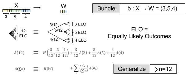
But suppose we choose a different bundling function 

For what function of 


Recall,


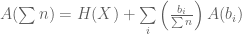

Hence,

![K \left[ \sum{p_i \log(\sum{n_i})} - \sum{p_i \log(n_i)} \right]](https://s0.wp.com/latex.php?latex=K+%5Cleft%5B+%5Csum%7Bp_i+%5Clog%28%5Csum%7Bn_i%7D%29%7D+-+%5Csum%7Bp_i+%5Clog%28n_i%29%7D+%5Cright%5D&bg=ffffff&fg=555555&s=0&c=20201002)
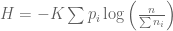
We have arrived at our definition of uncertainty, the entropy H(X):

To illustrate, consider a coin with bias p. Our uncertainty is maximized for a fair coin, p = 0.5, and smallest at p = 0.0 (certain tails) or 1.0 (certain heads).

Entropy vs Information
What is the relationship between uncertainty and information? To answer this, we must first understand information.
Consider the number of possible sentences in a book. Is this information? Two books contain exponentially more possible sentences than one book.
When we speak of information, we desire it to scale linearly with its length. Two books should contain approximately twice as much information.
If we take the logarithm of the possible messages

Recall that,

From here, we can show that entropy is expected information:


What does this discovery mean, though?
Imagine a device that produces 3 symbols, A, B, or C. As we wait for the next symbol, we are uncertain which symbol comes next. Once a symbol appears our uncertainty decreases, because we have received more information. Information is a decrease in entropy.
If A, B, and C occur at the same frequency, we should not be surprised to see any one letter. But if P(A) approaches 0, then we will be very surprised to see it appear, and the formula says I(X) approaches ∞. For the receiver of a message, information represents surprisal.
On this interpretation, the above formula becomes clear. Uncertainty is anticipated surprise. If our knowledge is incomplete, we expect surprise. But confident knowledge is “surprised by surprise”.
Conclusions
The great contribution of information theory lies in a measure for probabilistic uncertainty.
We desire this measure to be continuous, monotonic, and compositionally invariant. There is only one such function, the entropy H:
This explains why a broad distribution is more uncertain than one that is narrow.
Henceforth, we will view the words “entropy” and “uncertainty” as synonymous.
Related Works
- Shannon (1948). A Mathematical Theory of Communication
- Jaynes (1957). Information Theory and Statistical Mechanics
- Schneider (1995). Information theory primer
