Motivations

Bayesianism is a big deal. Here’s what the Stanford Encyclopedia had to say about it:

In the past decade, Bayesian confirmation theory has firmly established itself as the dominant view on confirmation; currently one cannot very well discuss a confirmation-theoretic issue without making clear whether, and if so why, one’s position on that issue deviates from standard Bayesian thinking.

What’s more, Bayesianism is everywhere:

• In philosophy of religion
• In general artificial intelligence
• In econometrics
• In cognitive biases
• In neuroscience
• Even drinking games !

In this post, I’ll introduce you to how it works in practice.

Probability Space

Humans are funny things. Even though we can’t produce randomness, we can understand it. We can even attempt to summarize that understanding, in 300 words or less. Ready? Go!

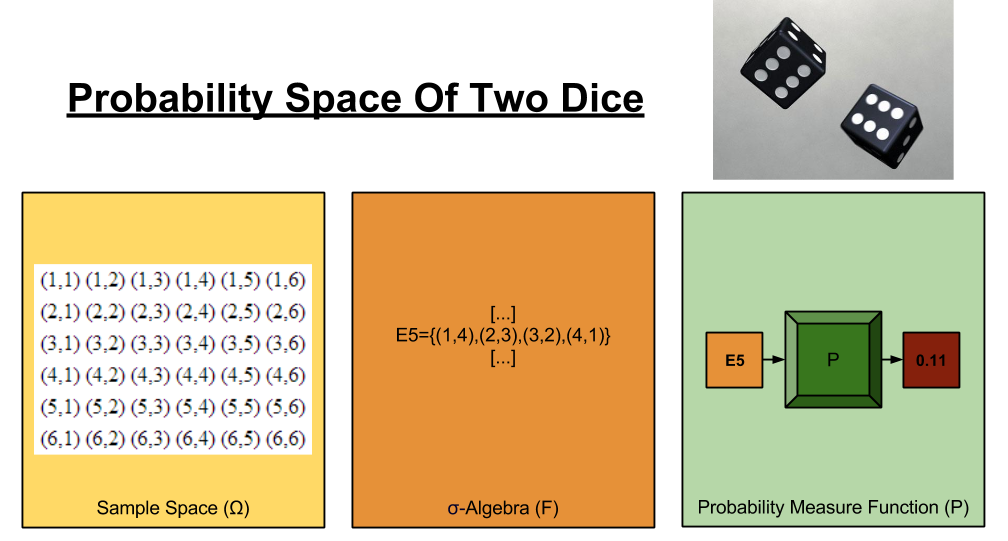
A probability space has three components:

1. Sample Space: A set of all possible outcomes, that could possibly occur. (Think: the ingredients)
2. σ-Algebra. A set of events, each of which contain at least one outcome. (Think: the menu)
3. Probability Measure Function. A set of probabilities, which convert events into numbers ranging from 0% to 100% (Think: the chef).

To illustrate, let’s carve out the probability space of two fair dice:

You remember algebra, and how annoying it was to use symbols that merely represented numbers? Statisticians get their jollies by terrorizing people with a similar toy, the random variable. The set of all possible values for a given variable is its domain.

Let’s define a discrete random variable called Happy.  We are now in a position to evaluate expressions like:

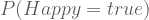
Such an explicit notation will get tedious quickly. Please remember the following abbreviations:

Okay, so let’s say we define the probability function that maps each manifestation of Happy’s domain to a number. What about when you take other information into account? Is your P(happy) going to be unaffected by learning, say, the outcome of the 2016 US Presidential Election? Not likely, and we’d like a tool to express this contextual knowledge. In statistics jargon, we would like to condition on this information. This information will be put on the RHS of the probability function, after a new symbol: |

Suppose I define a new variable, ElectionOutcome = { republican, democrat, green } Now, I can finally make intelligible statements about:

A helpful subvocalization of the above:

The probability of happiness GIVEN THAT the Green Party won the election.

Bayescraft

When I told you about conditioning, were you outraged that I didn’t mention outcome trees? No? Then go watch this (5min). I’ll wait.

Now you understand why outcome trees are useful. Here, then, is the complete method to calculate joint probability (“what are the chances X and Y will occur?”):

The above tree can be condensed into the following formula (where X and Y represent any value in these variables’ domain):

Variable names are arbitrary, so we can just as easily write:

But the joint operator (“and”) is commutative: . So we can glue the above equations together.

Since both of the equations above are equal to P(X, Y), we can glue them together:

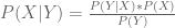
Dividing both sides by P(Y) gives us Bayes Theorem:

“Okay…”, you may be thinking, “Why should I care about this short, bland-looking equation?”

Look closer! Here, let me rename X and Y:

Let’s cast this back into English.

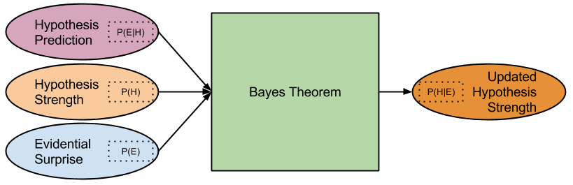
• P(Hypothesis) answers the question: how likely is it that my hypothesis is true?
• P(Hypothesis|Evidence) answers the question: how likely is my hypothesis, given this new evidence?
• P(Evidence) answers the question: how likely is my evidence? It is a measure of surprise.
• P(Evidence|Hypothesis) answers the question: if my hypothesis is true, how likely am I to see this evidence? It is a measure of prediction.

Shuffling around the above terms, we get:

We can see now that we are shifting, by some factor, from P(Hypothesis) to P(Hypothesis|Evidence). Our beginning hypothesis is now updated with new evidence. Here’s a graphical representation of this Bayesian updating:

DIY Inference

A Dream

Once upon a time, you are fast asleep. In your dream an angel appears, and presents you with a riddle:

“Back in the real world, right now, an email just arrived in your inbox. Is it spam?”

You smirk a little.

“This question bores me! You haven’t given me enough information!”
“Ye of little faith! Behold, I bequeath you information, for I have counted all emails in your inbox.”
“Revelation 1: For every 100 emails you receive, 78 are spam.”
“What is your opinion now? Is this new message spam?”
“Probably… sure. I think it’s spam.”

The angel glares at you, for reasons you do not understand.

“So, let me tell you more about this email. It contains the word ‘plans’.”
“… And how does that help me?”
“Revelation 2: The likelihood of ‘plans’ being in a spam message is 3%.”
“Revelation 3: The likelihood of it appearing in a normal message is 11%”
“Human! Has your opinion changed? Do you now think you have received the brainchild of some marketing intern?”

A fog of confusion and fear washes over you.

“… Can I phone a friend?”

You wake up. But you don’t stop thinking about your dream. What is the right way to answer?

Without any knowledge of its contents, we viewed the email as 78% likely to be spam. What changed? The word “plans” appears, and that word is more than three times as likely to occur in non-spam messages! Therefore, should we expect 78% to increase or decrease? Decrease, of course! But how much?

Math Goggles, Engage!

If you’ve solved a word problem once in your life, you know what comes next. Math!

Time to replace these squirmy words with pretty symbols! We shall build our house as follows:

• Let “Spam” represent a random variable. Its domain is { true, false }.
• Let “Plans” represent a random variable. Its domain is { true, false }

How might we cast the angel’s Revelations, and Query, to maths?

Word Soup	Math Diamonds
“R1: For every 100 emails you receive, 78 are spam.”	P(spam) = 0.78
“R2: The likelihood of ‘plans’ being in a spam message is 3%.”	P(plans|spam) = 0.03
“R3: The likelihood of it appearing in a normal message is 11%”	P(plans|¬spam) = 0.11
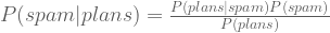
“Q: Is this message spam?”	P(spam|plans) = ?

Solving The Riddle

Of course, it is not enough to state a problem rigorously. It must be solved. With Bayes Theorem, we find that:

Do we know all of the terms on the right-hand side? No: we have not been given P(plans). How do we compute it? By a trick outside the scope of this post: marginalization. If we marginalize over Plans (i.e., sum over all instances of its domain), we spawn the ability able to compute P(E). In Mathese, we have:

P(plans,spam) and P(plans, ¬spam) represent joint probabilities that we can expand. Applying the Laws of Conditional Probability (given earlier), we have:

Notice we know the values of all the above variables except P(¬spam). We can use an axiom of probability theory to find it:

Word Soup	Math Diamonds
“Every variable had 100% chance of being something.”	P(X) + P(¬X) = 1.0.

Since the P(spam) is 0.78, we can infer that P(¬spam) is 0.22.

Now the fun part – plug in the numbers!

Take a deep breath. Stare at your result. Blink three times. Okay.

This new figure, 0.49, interacts with your previous intuitions in two ways.

1. It corroborates them: “plans” is evidence against spam, and 0.49 is indeed smaller than 0.78.
2. It sharpens them: we used to be unable to quantify how much the word “plans” would weaken our spam hypothesis.

The mathematical machinery we just walked through, then, accomplished the following:

Technical Rationality

We are finally ready to sketch a rather technical theory of knowledge.

In the above example, learning occured precisely once: on receipt of new evidence. But in real life we collect evidence across time. The Bayes learning mechanism, then, looks something like this:

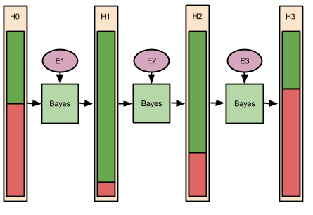
Let’s apply this to reading people at a party. Let H represent the hypothesis that some person you just met, call him Sam, is an introvert.

Suppose that 48% of men are introverts. Such a number represents a good beginning degree-of-confidence in your hypothesis. Your H0, therefore, is 48%.

Next, a good Bayesian would go about collecting evidence for her hypothesis. Suppose, after 40 minutes of discretely observing Sam, we see him retreat to a corner of the room, and adopt a “thousand yard stare’. Call this evidence E1, and our updated introversion hypothesis (H1) increases dramatically, say to 92%.

Next, we go over and engage Sam in a long conversation about his background. We notice that, as the conversation progresses, Sam becomes more animated and personable, not less. This new evidence E2 “speaks against” E1, and our hypothesis regresses (H2 becomes 69%).

After these pleasantries, Sam appears to be more comfortable with you. He leans forward and discloses that he just got out of a fight with his wife, and is battling a major headache. He also mentions regretting being such a bore at this party. With these explanatory data now available, your introversion hypothesis wanes. Sure, Sam could be lying, but the likelihood of that happening, in such a context, is lower than truth-telling. Perhaps later we will encounter evidence that induces an update towards a (lying) introvert hypothesis. But given the information we currently possess, our H3 rests at 37%.

Wrapping Up

Resources

In this post, I’ve taken a largely symbolic approach to Bayes’ Theorem. Given the extraordinary influence of the result, many other teaching strategies are available. If you’d like to get more comfortable with the above, I would recommend the following:

• Visualizing w/ probability mass
• Visualizing w/ Venn diagrams
• Visualizing w/ your own calculations

Takeaways

I have, by now, installed a strange image in your head. You can perceive within yourself a sea of hypotheses, each with their own probability bar, adjusting with every new experience. Sure, you may miscalculate – your brain is made of meat, after all. But you have a sense now that there is a Right Way to do reason, a normative bar that maximizes inferential power.

Hold onto that image. Next time, we’ll cast this inferential technique to its own epistemology (theory of knowledge), and explore the implications.