Intellectual History (2011-2014)

December 1, 2014December 4, 2014kevinbinz Leave a comment

An incomplete list, which only covers books and courses (not articles) I have fully consumed (vs. started)

2011

Your Inner Fish [Shubin (2008)]
Structure Of Scientific Revolutions [Kuhn]
Open Society and its Enemies [Popper]
Who Wrote The Bible? [Friedman]
Don’t Sleep There Are Snakes [Everett]
Cows, Pigs, Wars, Witches [Harris]
A History Of God [Armstrong]
Witchcraft, Oracles, Magic among Azande [Evans-Pritchard]
Why Zebras Don’t Get Ulcers [Sapolsky]
The Trouble With Testosterone [Sapolsky]
The Myth Of Sisyphus [Camus]
Dialogues Concerning Natural Religion [Hume]
[Lecture Series] Philosophy Of Death [Kagan]
[Lecture Series] Human Behavioral Biology [Sapolsky]
[Lecture Series] Yale: New Testament Literature & History [Martin]
[Lecture Series] Philosophy Of Science [Kasser]
[MOOC] Intro To AI

2012

Influence [Cialdini]
The Origin Of Consciousness and Breakdown of the Bicameral Mind [Jaynes]
Hero With A Thousand Faces [Campbell]
Beyond Good and Evil [Nietzsche]
Genealogy Of Morals [Nietzsche]
Lost Christianities [Ehrman]
The Modularity Of Mind [Fodor]
Five Dialogues: Euthyphro, Apology, Crito, Meno, Phaedo [Plato]
The Mind’s I [Dennett]
The Protestant Ethic and the Spirit Of Capitalism [Weber]
Interpretation Of Dreams [Freud]
Good and Real [Drescher]
In Two Minds [Evans, Frankish]
Thinking Fast and Slow [Kahneman (2011)]
Working Memory: Thought and Action [Baddeley]
Philosophy Of Mind [Jaworski]
[Lecture Series] Brain Structure And Its Origins [Schneider]
[Lecture Series] Justice [Sandel]
[MOOC] Machine Learning [Ng]
[MOOC] Health Policy & The ACA
[MOOC] Networked Life

2013

Evolutionary Physchology 4th edition [Buss (2011)]
Vision [Marr (1982)]
The Visual Brain in Action [Milner, Goodale (2006)]
Foundations Of Neuroeconomic Analysis [Glimcher]
Flow: The Psychology Of Optimal Experience [Csikszentmihalyi]
Architecture Of Mind [Carruthers (2006)]
[UW Course] CSEP524 Parallel Computation [Chamberlain]
[UW Course] CSEP514 Natural Language Processing [Zettlemoyer]
[UW Course] CSEP576 Computer Vision [Farhadi]

2014

The Conservative Mind [Kirk]
Guns, Gems, and Steel [Diamond]
Semiotics For Beginners [Chandler]
Rationality and the Reflective Mind [Stanovitch]
The Robot’s Rebellion [Stanovitch]
The Righteous Mind [Haidt]
The Selfish Gene [Dawkins]
The Better Angels Of Our Nature [Pinker]
The Illusion Of Conscious Will [Wegner (2003)]
[UW Course] CSEP590 Molecular and Neural Computation [Seelig]
[UW Course] CSEP573 Artificial Intelligence [Farhadi]
[UW Course] EE512A Advanced Inference In Graphical Models [Bilmes]

Tunneling Into The Soup

September 7, 2014September 7, 2014kevinbinz Leave a comment

Table Of Contents

Context
Bathing In Radiation
Our Photoreceptive Hardware
The Birthplace Of Human-Visibility
Takeaways

Context

In Knowledge: An Empirical Sketch, I left you with the following image of perceptual tunneling:

Today, we will explore this idea in more depth.

Bathing In Radiation

Recall what you know about the nature of light:

Since h and c are just constants, the relation becomes very simple: energy is inversely proportional to wavelength. Rather than identifying a photon by its energy, then, let’s identify it by its wavelength. We will do this because wavelength is easier to measure (in my language, we have selected a measurement-affine independent variable).

So we can describe one photon by its wavelength. How about billions? In such a case, it would be useful to draw a map, on which we can locate photon distributions. Such a photon map is called an electromagnetic spectrum.

With this background knowledge in place, we can explore a photon map of solar radiation: what types of photons strike the Earth from the Sun?

This image is rather information-dense. Let’s break it down.

Compare the black curve to the yellow distribution. The former represents the difference between an idealized energy radiator (a black body), whereas the latter represents the actual transmission characteristics of the sun. As you can see, while the black body abstraction does not perfectly model the idiosyncrasies of our Sun, it does a pretty good job “summarizing” the energy output of our star.

Next, compare the yellow distribution to the red distribution. The former represents solar radiation before it hits our atmosphere, the latter represents solar radiation after it hits our atmosphere (when it strikes the Earth). As you can see, at some wavelengths light passes through the atmosphere easily (red ~= yellow; call this atmospheric lucidity) whereas at other wavelengths, the atmosphere absorbs most of the photons (red << yellow; call this atmospheric opacity).

These different responses to different energy light does not occur at random, of course. Rather, the chemical composition of the atmosphere causes atmospheric opacity. Ever hear the meme “the ozone layer protects us from UV light”? Well, here is that data underlying the meme (see the “O3” marker at the 300 nm mark?). Other, more powerful but less well-known, effects can be seen in the above spectrum, which characterize the shielding effects of water vapor, carbon dioxide, and oxygen onto the spectra.

Our Photoreceptive Hardware

Your eyes house two types of photoreceptive cell: the rod and the cone.

Rods are tuned towards performing well in low-light conditions. After roughly 30 minutes in the dark, everything is ready for optical stimulation. In this “dark-adapted” state, the visual system is amazingly sensitive. A single photon of light can cause a rod to trigger. You will see a flash of light if as few as seven rods absorb photons at one time.

Cones, on the other hand, excel in daylight. They also underwrite the experience of color (a phenomenon we will discuss next time). Now, unless you are a tetrachromat mutant, your eyes contain three kinds of cone:

16% blue cones
10% green cones
74% red cones

Below are the absorption spectra. Please note that, while not shown, rods manifest a similar spectrum: they reside between the blue and green curves , with a peak receptivity is 498 nm.

It is important to take the above in context of the cone’s broader function. By virtue of phototransductive chemical processes, sense organs like the cone accept photons matching the above spectrum as input, and thereby facilitate the production of spike trains (neural code) as system output.

The Birthplace Of Human-Visibility

We now possess two spectra: one for solar radiation, and one for photoreceptor response profile. Time to combine spectra! After resizing the images to achieve scale consistency, we arrive at the following:

Peak solar radiation corresponds to cone spectrum! Why should this be? Well, recall the purpose of vision in the first place. Vision is an evolutionary adaptation that extracts information from the environment & makes it available to the nervous system of its host. If most photon-mediated information is happening at the 450-700 nm energy level, should we really be so surprised to learn that our eyes have adapted to this particular range?

Notice that we drew two dotted lines around the intersection boundaries. We have now earned the right to use a name. Let us name photons that reside within the above interval, visible light. Then,

Let “ultraviolet light” represent photons to the left of the interval (smaller wavelengths, higher energy)
Let “infrared light” represent photons to the right of the interval (longer wavelengths, lower energy)

We have thus stumbled on the definition of visibility. Visibility is not an intrinsic physical property, like charge. Rather, it is human invention: the boundary at which our idiosyncratic photoreceptors carve into the larger particle soup.

Takeaways

We have now familiarized ourselves with the mechanism of tunneling. Perceptual tunneling occurs when sense organ transduces some slice of the particle soup of reality. In vision, photoreceptors cells transduce photons within the 450-700 nm energy band into the neural code.

With this precise understanding of transduction, we begin to develop a sense of radical contingency. For example,

Ever wonder what would happen if the human eye also contained photoreceptors on the 1100 nm range? The human umwelt As you heat a fire up, for example, you would see tendrils of flame brighten, then vanish, then reappear. I suspect everyday language would feature “bright-visible” and “dim-visible”
Consider what would have happened if, during our evolution, the solar radiation spectrum if the sun had been colder than 5250 degrees Celsius. The black-body idealized spectrum of the sun would shift, and its peak would move towards the right. The actual radiation signature of the sun (yellow distribution) would follow. Given how precisely the rods in our eyes “found” the band of peak emitted energy in this universe, in that world, it seems likely that we would be wearing different photoreceptors with an absorption signature better calibrated to the the new information. Thus, we have a causal link between the temperature of the Sun and the composition of our eyeballs.

I began this post with a partial quote from Metzinger. Here is the complete quote:

The evening sky is colorless. The world is not inhabited by colored objects at all. It is just as your physics teacher in high school told you: Out there, in front of your eyes, there is just an ocean of electromagnetic radiation, a wild and raging mixture of different wavelengths. Most of them are invisible to you and can never become part of your conscious model of reality. What is really happening is that your brain is drilling a tunnel through this inconceivably rich physical environment and in the process painting the tunnel walls in various shades of color. Phenomenal color. Appearance.

Next time, we’ll explore the other half of Metzinger’s quote: “painting the tunnel walls in various shades of color, phenomenal color”…

Movement Forecast: Effective Availabilism

August 19, 2014August 24, 2014kevinbinz Leave a comment

Table Of Contents

The Availability Cascade
Attentional Budget Ethics
Effective Availabilism
Why Quantification Matters
Cascade Reform Technologies
Takeaways

The Availability Cascade

The following questions pop up in my Facebook feed all the time.

Why is mental illness, addiction, and suicide only talked about when somebody famous succumbs to their demons?

Why do we only talk about gun control when there is a school shooting?

What is the shape of your answer? Mine begins with a hard look at the nature of attention.

Attention is a lens by which our selves perceive the world. The experience of attention is conscious. However, the control of attention – where it lands, how long it persists – is preconscious. People rarely think to themselves: “now seems an optimal time to think about gun control”. No, the topic of gun control simply appears.

When we pay attention to attention, its flaws become visible. Let me sketch two.

The preconscious control of attention is famously vulnerable to a wide suite of dysrationalia. Like transposons parasitizing your DNA, beliefs parasitize your semantic memory by latching onto your preconscious attention-control software. This is why Evans-Pritchard was so astonished in his anthropological survey of Zande mysticism. This is why your typical cult follower is pathologically unable to pay attention to a certain set of considerations. The first flaw of the attentional lens is that it is a biasing attractor.
Your unconscious mind is subject to the following computational principle: what you see is all there is. This brings us the availability heuristic, the cognitive shortcut your brain uses to travel from “this was brought to mind easily” to “this must be important”. The attentional lens is that the medium distorts its contents. This is nicely summed up in the proverb, “nothing in life is as important as you think it is, while you are thinking about it.” The second flaw of the attentional lens is that bound in a positive feedback loop to memory (“that which I can recall easily, must be important, leads me to discuss more, is something I recall even more easily”).

My treatment of this positive feedback loop was at the level of individual. But that same mechanism must also promote failures at the level of social network. The second flaw writ large – the rippling eddies of attentional currents (as captured by services like Google News) – are known as availability cascades. And thus we have provided a cognitive reason why our social atmosphere disproportionately discusses gun control when school shootings appear in the news.

In electrical engineering, positive feedback typically produces runaway effects: a circuit “hits the rails” (draws maximum current from its power source). What prevents human cognition from doing likewise, from becoming so fixated on one particular memory-attention loop that it cannot escape? Why don’t we spend our days and our nights dreaming of soft drinks, fast food, pharmaceuticals? I would appeal to human boredom as a natural barrier to such a runaway effect.

Attentional Budget Ethics

We have managed to rise above the minutia, and construct a model of political discourse. Turn now to ethics. How should attention be distributed? When is the right time to discuss gun control, to study health care reform, to get clear on border control priorities?

The response profile of such a question is too diverse to treat here, but I would venture most approaches share two principles of attentional budgets:

The Systemic Failure Principle. If a system performance fails to meet some arbitrary criteria of success, that would be an argument for increasing its attentional budget. For example, perhaps the skyrocketing costs of health care would seem to call for more attention than other, relatively more healthy, sectors of public life.
The Low Hanging Fruit Principle. If attention is likely to produce meaningful results, that would be an argument for increasing its attentional budget. For example, perhaps not much benefit would come from a national conversation about improving our cryptographic approaches to e-commerce.

Despite how shockingly agreeable these principles are, I have a feeling that different political parties may yet disagree. In a two party system, for example, you can imagine competing attentional budgets as follows:

Interpret “attentional resources” in a straightforward (measurement-affine) way: let it represent the number of hours devoted to public discussion.

This model of attentional budgets requires a bit more TLC. Research-guiding questions might include:

How ought we model overlapping topics?
Should budget space be afforded for future topics, topics not yet conceived?
Could there be circumstances to justify zero attention allocation?
Is it advisable to leave “attentional budget creation” topics out of the budget?
How might this model be extended to accomodate time-dependent, diachronic budgeting?

Effective Availibilism

Let us now pull together a vision of how to transcend the attentional cascade.

In our present condition, even very intelligent commentators must resort to the following excuse of a thought: “I have a vague sense that our society is spending too much time on X. Perhaps we shouldn’t talk about it anymore”.

In our envisioned condition, our best political minds would be able to construct the following chain of reasoning: “This year, our society has spent three times more time discussing gun control than discussing energy independence. My attentional budget prescribes this ratio to be closer to 1:1. Let us think of ways to constrain these incessant gun-control availability cascades.”

In other words, I am prophesying the emergence of an effective availabilism movement, in ways analogous to effective altruism. Effective availabilist groups would, I presume, primarily draw from neuropolitical movements more generally.

Notice how effective availabilism relies on, and comes after, of publically-available psychometric data. And this is typical: normative movements often follow innovations in descriptive technology.

Why Quantification Matters

Policy discussions influence votes which affect lives. Despite the obvious need for constructive discourse, a frustrating amount of political exchanges are content-starved. I perceive two potential solutions for this failure of our democracy:

Politics is a mind-killer. By dint of our evolutionary origins, our brains do not natively excel at political reasoning. Group boundaries matter more than analyses, arguments are soldiers. But these are epistemic failure modes. Policy debates should not appear one-sided. Movements to establish the cognitive redemption of politics are already underway. See, for example, Jonathon Haidt’s http://www.civilpolitics.org/ (“educating the public on evidence-based methods for improving inter-group civility”)
Greasing policy discussions with data would facilitate progress. One of my favorite illustrations of this effect is biofeedback: if you give a human being a graphical representation of her pulse, the additional data augments the brains ability to reason – biofeedback patients are even able to catch their breath faster. In the same way, improving our data streams gives hope of transcending formerly-intractable social debates.

The effective availabilism movement could, in my view, accelerate this second pathway.

Cascade Reform Technologies

It seems clear that availability cascades are susceptible to abuse. Many advertisers and political campaigns don’t execute an aggregated optimization across our national attentional profile. Instead, they simply run a maximization algorithm on their topic of interest (“think about my opponent’s scandal!”).

With modern-day technology (polls, trending Twitter tags, motive abduction, self-monitoring), noticing attentional budget failures can be tricky. With the above technology in place, even subtle attentional budget failures will be easily detectable. We have increased our supply of failures, but how might effective availabilists increase demand (open vectors of reform towards availability cascade failure modes)?

The first, obvious, pathway is to use the same tool – attentional cascades – to counterbalance. If gun control is getting too much attention, effective availabilists will strive to push social media towards a discussion of e.g., campaign finance reform. They could, further, use psychometric data to evaluate whether they have overshot (SuperPACs are now too interesting), and to adjust as necessary.

Other pathways towards reform might be empirically-precise amplification of boredom circuits. Recruit the influential to promote the message that “this topic has been talked to death” could work; as could the targeted use of satire.

Takeaways

Pay more attention to the quiet whispers of your mind. “Haven’t I heard about this enough” represents an undiscovered political movement.
Social discourse is laced with the rippling tides of availability cascades, and are at present left to their mercy.
As hard psychometric data makes its way towards public accessibility, a market of normative attentional budgets will arise.
The business of pushing current attentional profiles towards normative budgets will become the impetus of effective availabilism movements.
A cottage industry of cognitive technologies to achieve these ends will thereafter crystallize and mature.

Fermions: Meat In Our Particle Soup

July 27, 2014March 20, 2017kevinbinz Leave a comment

Part Of: Demystifying Physics sequence
Prerequisite Post: An Introduction To Energy
Content Summary: 2100 words, 21 min reading time.

Prerequisite Mindware

Today, we’re going to go spelunking into the fabric of the cosmos! But first, some tools to make this a safe journey.

Energy Quanta

As we saw in An Introduction to Energy,

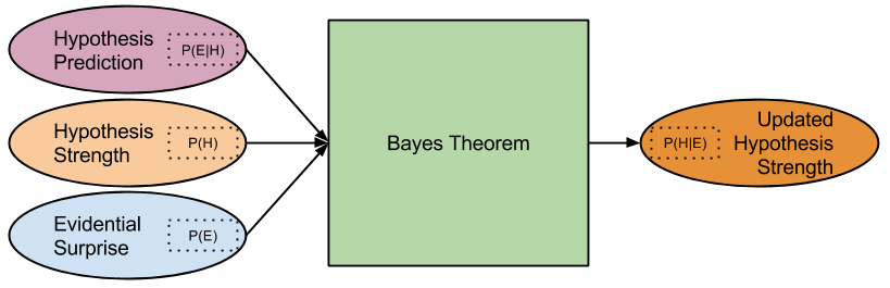
Energy is the hypothesis of a hidden commonality behind every single physical process. There are many forms of energy: kinetic, electric, chemical, gravitational, magnetic, radiant. But these forms are expressions of a single underlying phenomena.

Consider the analogy between { electrons spinning around protons } and { planets spinning around stars }. In the case of planets, the dominant force is gravitational. In the case of the atom, the dominant force is electromagnetic.

But the analogy strength of the above is weak. In contrast to gravitational acceleration, an accelerating electric charge emits electromagnetic waves. Thus, we would expect an orbiting charge to steadily lose energy and spiral into the nucleus, colliding with it in a fraction of a second. Why have atoms not gone extinct?

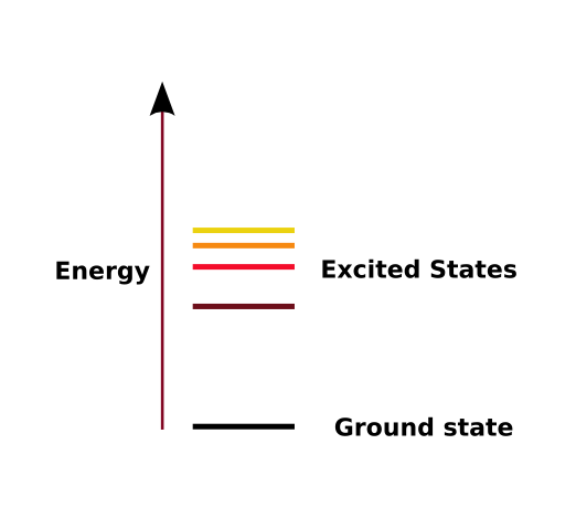
To solve this problem, physicists began to believe that in some situations, energy cannot be lost. Indeed, they abandoned the intuitive idea that energy is continuous. On this new theory, at the atomic level energy must exist in certain levels, and never in between. Further, at one particular energy level, something we will call the ground state, an electron may never lose energy.

Antiparticles

Let’s talk about antiparticles. It’s time to throw out your “science fiction” interpretive lens: antiparticles are very real, and well-understood. In fact, they are exactly the same as normal particles, except charge is reversed. So, for example, an antielectron has the same mass and spin as an electron, but instead carries a positive charge.

Why does the universe contain more particles than antiparticles? Good question. 😛

Meet The Fermions

Nature Up Close

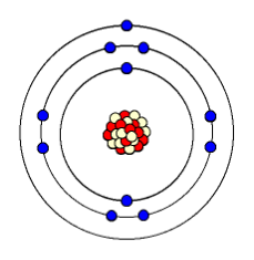
Consider this thing. What would you name it?

One name I wouldn’t select is “indivisible”. But that’s what the “atom” means (from the Greek “ἄτομος”). Could you have predicted the existence of this misnomer?

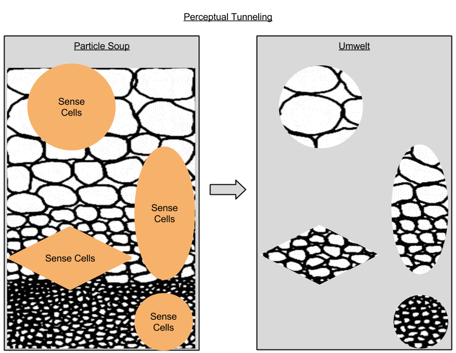
As I have discussed before, human vision can capture only a small subset of physical reality. Measurement technology is a suite of approaches that exploit translation proxies, the ability to translate extrasensory phenomena into a format amenable to perception. Our eyes cannot perceive atoms, but the scanning tunneling microscope translates atomic structures to scales our nervous systems are equipped to handle.

Let viable translation distance represent the difference in scale between human perceptual foci and the translation proxy target. Since translation proxies are facilitated through measurement technology, which is in turn driven by scientific advances, it follows that we ought to expect viable translation distance to increase over time.

We now possess a straightforward explanation of our misnomer. When “atom” was coined, its referent was the product of that time’s maximum viable translation distance. But technology has since moved on, and we have discovered even smaller elements. Let’s now turn to the state of the art.

Beyond The Atom

Reconsider our diagram of the atom. Do you remember the names of its constituents? That’s right: protons, neutrons, and electrons. Protons and neutrons “stick together” in the nucleus, electrons “circle around”.

Our building blocks of the universe so far: { protons, neutrons, electrons }. By combining these ingredients in all possible ways, we can reconstruct the periodic table – all of chemistry. Our building blocks are – and must be – backwards compatible. But are these particles true “indivisibles”? Can we go smaller?

Consider the behavior of the electrons orbiting the nucleus. After fixing one theoretical problem (c.f., Energy Levels section above), we now can explain why electrons orbit the nucleus: electromagnetic attraction (“opposites attract”). But here is a problem: we have no such explanation for the nucleus. If “like charges repel”, then the nucleus must be something like holding the same poles of a magnet close together: you can do it, but it takes a lot of force. What could possibly be keeping the protons in the nucleus together?

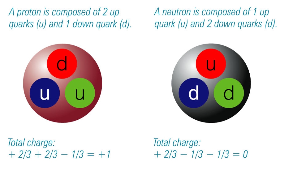
Precisely this question motivated a subsequent discovery: electrons may well be indivisible, but protons and neutrons are not. Protons and neutrons are instead composite particles made out of quarks. Quarks like to glue themselves together by a new force, known as the strong force. This new type of force not only explains why we don’t see quarks by themselves, it also explains the persistence of the nucleus.

The following diagram (source) explains how quarks comprise protons and neutrons:

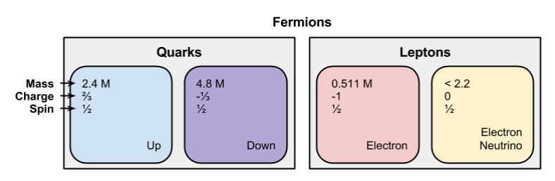
Okay, so our new set of building blocks are: { electron, up, down }. With a little help from some new mathematics – quantum chromodynamics – we can again reconstitute chemistry. biology, and beyond.

Please notice how some of our building blocks are more similar than others: the up and down particle comprise particles with charge divisible by three, the electron particle carries an integer charge. Let us group like particles together.

Call up and down particles part of the quark family.
Call electrons part of the lepton family.

Neutrinos

So far in this article, we’ve gestured towards gravitation and electromagnetism. We’ve also introduced the strong force. Now is the time to discuss Nature’s last muscle group, the weak force.

A simple way to bind the weak force to your experience: consider what you know about radioactive material. The types of atoms that are generated in, to pick one source, nuclear power do not behave like other atoms. They emit radiation, they decay. Ever heard of the “half-life” of a material? That term defines how long is takes for half of an unstable radioactive material to decay into a more stable form. For example, { magnesium-23 → sodium-23 + antielectron }.

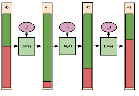
Conservation of energy dictates that such decay reactions must preserve energy. However, when you actually calculate the energetic content of decay process given above, you find a mismatch. And so, scientists were confronted with the following dilemma: either reject conservation of energy, or posit the existence of an unknown particle to “balances the books”. Which would you chose?

The scientific community began to speculated that a fourth type of fermion existed, even with an absence of physical evidence. And they found it 26 years later, in 1956.

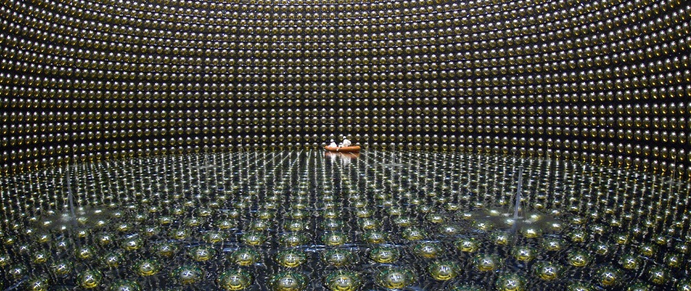
Why did it take relatively longer to discover this fourth particle? Well, these hypothesized neutrinos do not carry an electric charge or a color charge. As such, they only interact with other particles via the weak force (which has a very short range) and the atomic force (which is 10^36 times less powerful than electromagnetic force). Due to these factors, neutrinos such as those generated by the Sun pass through the Earth undetected. In fact, in the time it takes you to read this sentence, hundreds of billions of neutrinos have passed through every cubic centimeter of your body without incident. Such weak interactivity explains the measurement technology lag.

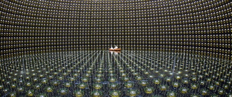
Are you sufficiently creeped out by how many particles pass through you undetected? 🙂 If not, consider neutrino detectors. Because of their weak interactivity, our neutrino detectors must be large, and buried deep inside the earth (to shield from “noise” – more common particle interactions). Here we see a typical detector, with scientists inspecting their instruments in the center, for contrast:

The Legos Of Nature

Here, then, is our picture of reality:

Fermions- One Generation

Notice that all fermions have spin ½; we’ll return to this fact later.

A Generational Divide

Conservation of energy is a thing, but conservation of particles is not. Just as particles spontaneously “jump” energy levels, sometimes particles morph into different types of particles, in a way akin to chemical reactions. What would happen if we were to pump a very large amount of energy into the system, say by striking an up quark with a high-energy photon? Must the output energy be expressed as hundreds of up quarks? Or does nature have a way to “more efficiently” spend its energy budget?

It turns out that you can: there exist particles identical to these four fermions with one exception: they are more massive. And we can pull this magic trick once more, and find fermions even heavier than these fermions. To date, physicists have discovered three generations of fermions:

Fermions- Three Generations

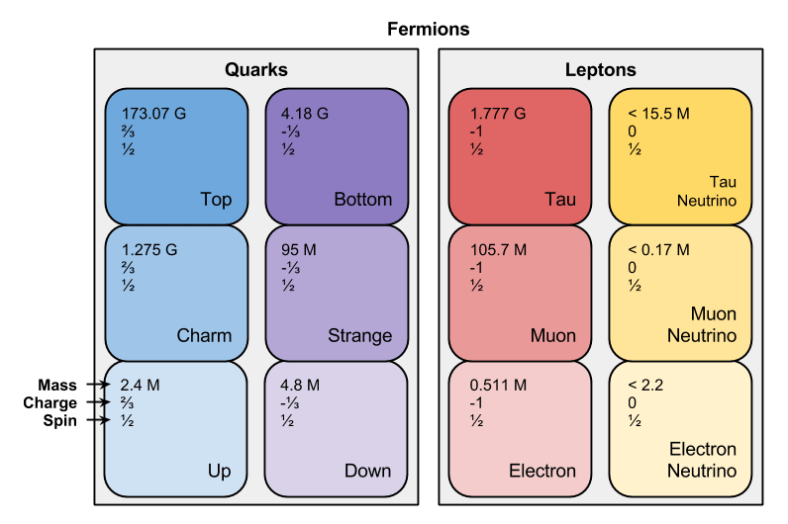
The latter generation took lots of time to “fill in” because you only see them in high-energy situations. Physicists had to close the translation distance gap, by building bigger and bigger particle accelerators. The fermion with the highest mass – the Top quark – was only discovered in 1995. Will there be a fourth generation, will we discover some upper bound on fermion generations?

Good question.

Even though we know of three generations, in practice only the first generation “matters much”. Why? Because the higher-energy particles that comprise the second and third generations tend to be unstable: give them time (fractions of a second, usually), and they will spontaneously decay – via the weak force – back into first generation forms. This is the only reason why we don’t find atomic nuclei orbited by tau particles.

Towards A Mathematical Lens

General & Individual Descriptors

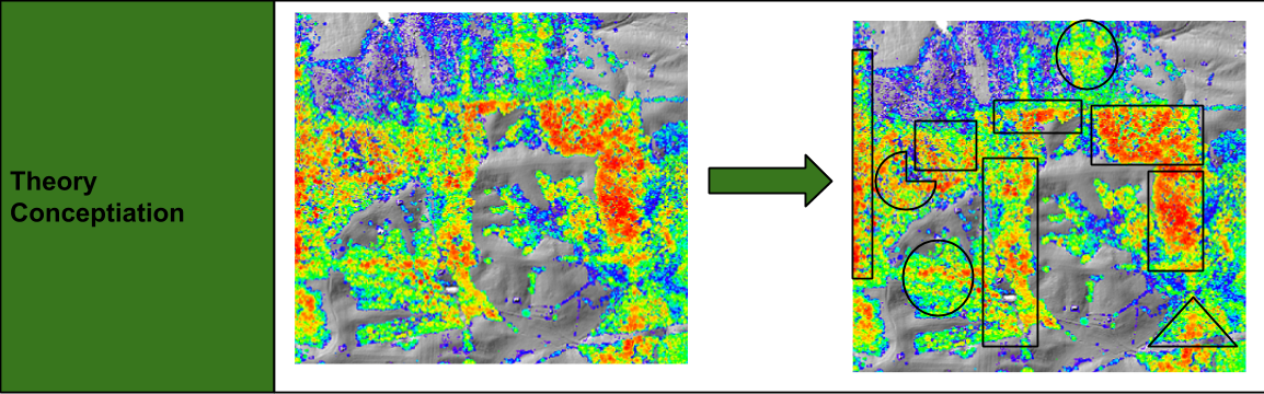
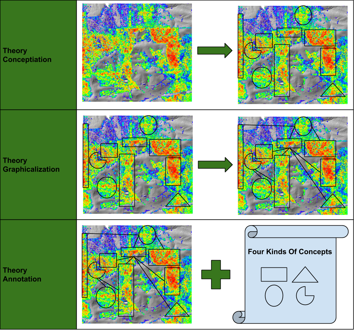
The first phase of my lens-dependent theorybuilding triad I call conceptiation: the art of carving concepts out of a rich dataset. Such carving must be heavily dependent on descriptive dimensions: quantifiable ways that an entity may differ from one another.

For perceptual intake, the number of irreducible dimensions may be very large. However, for particles, this set is surprisingly small. There is something distressingly accurate in the phrase “all particles are the same”.

Each type of fermion is associated with one unique value for the following properties (particle-generic properties):

mass (m)
electric charge (e)
spin (s)

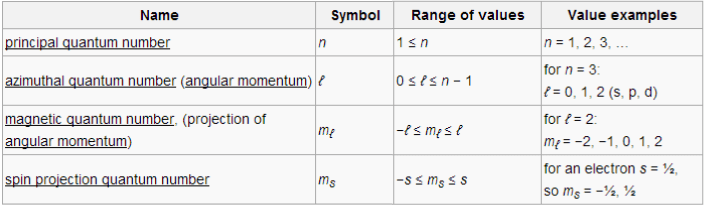
Fermions may differ according to their quantum numbers (particle-specific properties). For an electron, these numbers are:

principal. This corresponds to the energy level of the electron (c.f., energy level discussion)
azimuthal. This corresponds to the orbital version of angular momentum (e.g., the Earth rotating around the Sun). These numbers correspond to the orbitals of quantum chemistry (0, 1, 2, 3, 4, …) ⇔ (s, p, d, f, g, …); which helps explain the orbital organization of the periodic table.
magnetic. This corresponds to the orientation of the orbital.
spin projection. This corresponds to the “spin” version of angular momentum (e.g., the Earth rotating around its axis). Not to be confused with spin, this value can vary across electrons.

Quantum numbers are not independent; their ranges hinge on one another in the following way:

Statistical Basis

With our fourth building block in place, we are in a position to answer the question: what does the particulate basis of matter have in common?

All elementary particles of matter we have seen have spin ½. By the Spin-statistics Theorem, we must associate all such particles with Fermi-Dirac statistics. Let us name all particles under this statistics – all particles we have seen so far – “fermions”. It turns out that this statistical approach generates a very interesting property known as the Pauli Exclusion Principle. The Pauli Exclusion Principle states, roughly, that two particles cannot share the same quantum state.

Let’s take an example: consider a hydrogen atom with two electrons. Give this atom enough time, and both electrons will be on its ground state, n=1. What happens if the hydrogen picks up an extra electron, in some chemical process? Can this third electron also enter the ground state?

No, it cannot. Consider the quantum numbers for our first two electrons: { n=1, l=0, m_l=0, m_s=1/2 } and { n=1, l=0, m_l=0, m_s=-1/2 }. Given the range constraints given above, there are no other unique descriptors for an electron with n=1. Since we cannot have two electrons with the same quantum numbers, the third electron must come to rest at the next highest energy level, n=2.

The Pauli Exclusion Principle has several interesting philosophical implications:

Philosophically, this means that if two things have the same description, then they cannot be two things. This has interesting parallels to the axiom of choice in ZFC, which accommodates “duplicate” entries in a set by conjuring some arbitrary way to choose between them.
Practically, the Pauli Exclusion Principle is the only thing keeping your feet from sinking into the floor right now. If that isn’t a compelling demonstration of why math matters, then I don’t know what is.

Composite Fermions

In this post, we have motivated the fermion particulate class by appealing to discoveries of elementary particles. But then, when we stepped back, we discovered that the most fundamental attribute of this class of particles was its subjugation to Fermi-Dirac statistics.

Can composite particles have spin-½ as well as these elementary particles? Yes. While all fermions considered in this post are elementary particles, that does not preclude composite particles from membership.

What Fermions Mean

In this post, we have done nothing less than describe the basis of matter.

But are fermions the final resolution of nature? Our measurement technology continues to march on. Will our ability to “zoom in” fail to produce newer, deeper levels of reality?

Good questions.

Knowledge: An Empirical Sketch

July 22, 2014July 22, 2014kevinbinz Leave a comment

Table Of Contents

Introduction
- All The World Is Particle Soup
- Soup Texture
Perceptual Tunnels
- On Resolution
- Sampling
- Light Cones, Transduction Artifacts, Translation Proxies
The Lens-dependent Theorybuilding Triad
- Step One: Conceptiation
- Step Two: Graphicalization
- Step Three: Annotation
- Putting It All Together: The Triad
Conclusion
- Going Meta
- Takeaways

Introduction

All The World Is Particle Soup

Scientific realism holds that the entities scientists refer to are real things. Electrons are not figments of our imagination, they possess an existence independent of your mind. What does it mean for us to view particle physics with such a lens?

Here’s what it means: every single thing you see, smell, touch… every vacation, every distant star, every family member… it is all made of particles.

This is an account of how the nervous system (a collection of particles) came to understand the universe (a larger collection of particles). How could Particle Soup ever come to understand itself?

Soup Texture

Look at your hand. How many types of particles do you think you are staring at? A particle physicist might answer: nine. You have four first-generation fermions (roughly, particles that comprise matter) and five bosons (roughly, particles to carry force). Sure, you may get lucky and find a couple exotic particles within your hand, but such a nuance would not detract from the morale to the story: in your hand, the domain (number of types) of particles is very small.

Look at your hand. How large a quantity of particles do you think you are staring at? The object of your gaze is a collection of about 700,000,000,000,000,000,000,000,000 (7.0 * 10^26) particles. Make a habit about thinking in this way, and you’ll find a new appreciation for the Matrix Trilogy. 🙂 In your hand, the cardinality (number of tokens) of particles is very large.

These observations generalize. There aren’t many kinds of sand in God’s Sandbox, but there is a lot of it, with different consistencies across space.

Perceptual Tunnels

On Resolution

Consider the following image. What do you see?

Your eyes filter images at particular frequencies. At this default human frequency, your “primitives” are the pixelated squares. However, imagine being able to perceive this same image at a lower resolution (sound complicated? move your face away from the screen :P). If you do this, the pixels fade, and a face emerges.

Here, we learn that different resolution lens may complement one another, despite their imaging the same underlying reality. In much the same way, we can enrich our cognitive toolkit by examining the same particle soup with different “lens settings”.

Sampling

By default, the brain does not really collect useful information. It is only by way of sensory transductor cells – specialized cells that translate particle soup into Mentalese – that the brain gains access to some small slice of physical reality. With increasing quantity and type of these sensory organs, the perceptual tunnel burrowed into the soup becomes wide enough to support a lifeform.

Another term for the perceptual tunnel is the umwelt. Different biota experience different umwelts; for example, honeybees are able to perceive the Earth’s magnetic field as directly as we humans perceive the sunrise.

Perceptual tunneling may occur at different resolutions. For example, your proprioceptive cells create signals only on the event of coordinated effort of trillions and trillions of particles (e.g., the wind pushes against your arm). In contrast, your vision cells create signals at very fine resolutions (e.g., if a single photon strikes your photoreceptor, it will fire).

Light Cones, Transduction Artifacts, Translation Proxies

Transduction is a physically-embedded computational process. As such, it is subject to several pervasive imperfections. Let me briefly point towards three.

First, nature precludes the brain from the ability to sample from the entirety of the particle soup. Because your nervous system is embedded within a particular spatial volume, it is subject to one particular light cone. Since particles cannot move faster than the speed of light, you cannot perceive any non-local particles. Speaking more generally: all information outside of your light cone is closed to direct experience.

Second, the nervous system is an imperfect medium. It has difficulty, for example, representing negative numbers (ever try to get a neuron firing -10 times per second?). Another such transduction artifact is our penchant for representing information in a comparative, rather than absolute, format. Think of all those times you have driven on the highway with the radio on: when you turn onto a sidestreet, the music feels louder. This experience has nothing at all to do with an increased sound wave amplitude: it is an artifact of a comparison (music minus background noise). Practically all sensory information is stained by this compressive technique.

Third, perceptual data may not represent the actual slice of the particle soup we want. To take one colorful example, suppose we ask a person whether they perceived a dim flashing light, and they say “yes”. Such self-reporting, of course, represents sensory input (in this case, audio vibrations). But this kind of sensory information is a kind of translation proxy to a different collection of particles we are interested in observing (e.g., the activity of your visual cortex).

This last point underscores an oft-neglected aspect of perception: it is an active process. Our bodies don’t just sample particles, they move particles around. Despite the static nature of our umwelt, our species has managed to learn ever more intricate scientific theories in virtue of sophisticated measurement technology; and measurement devices are nothing more than mechanized translation proxies.

The Lens-dependent Theorybuilding Triad

Step One: Conceptiation

Plato once describes concept acquisition as “carving nature at its joints”. I will call this process (constructing Mentalese from the Soup) theory conceptiation.

If you meditate on this diagram for a while, you will notice that theory conceptiation is a form of compression. Acccording to Kolmogorov information theory, the efficacy of compression hinges on how many patterns exist within your data. This is why you’ll find leading researchers claiming that:

Compression and Artificial Intelligence are equivalent problems

A caveat: concepts are also not carved solely from perception; as one’s bag of concepts expands, such pre-existent mindware exerts an influence on the further carving up of percepts. This is what the postmoderns attribute to hermeneutics, this is the root of memetic theory, this is what is meant by the nature vs. nurture dialogue.

Step Two: Graphicalization

Once the particle soup is compressed into a set of concepts, relations between these concepts are established. Call this process theory graphicalization.

If I were ask you to complete the word “s**p”, would you choose “soap” or “soup”? How would your answer change if we were to have a conversation about food network television?

Even if I never once mention the word “soup”, you become significantly more likely to auto-complete that alternative after our conversation. Such priming is explained through concept graphs: our conversation about the food network activates food-proximate nodes like “soup” much more strongly than graphically distant nodes like “soap”.

Step Three: Annotation

Once the graph structure is known, metagraph information (e.g., “this graph skeleton occurs frequently”) is appended. Such metagraph information is not bound to graphs. Call this process theory annotation.

We can express a common complaint about metaphysics thusly: theoretical annotation is invariant to changes in conceptiation & graphicalization results. In my view (as hinted at by my discussion of normative therapy) theoretical annotation is fundamentally an accretive process – it is logically possible to generate an infinite annotative tree; this is not seen in practice because of the computational principle of cognitive speed limit (or, to make a cute analogy, the cognition cone).

Putting It All Together: The Triad

Call the cumulative process of conceptiation, graphicalization, and annotation the lens-dependent theorybuilding triad.

Conclusion

Going Meta

One funny thing about theorybuilding is how amenable it is to recursion. Can we explain this article in terms of Kevin engaging in theorybuilding? Of course! For example, consider the On Resolution section above. Out of all possible adjectives used to describe theorybuilding, I deliberately chose to focus my attention on spatial resolution. What phase of the triad does that sound like to you? Right: theory conceptiation.

Takeaways

This article does not represent serious research. In fact, its core model – the lens-dependent theorybuilding triad – cites almost no empirical results. It is a toy model designed to get us thinking about how a cognitive process can construct a representation of reality. Here is an executive summary of this toy model:

Perception tunneling is how organisms begin to understand the particle soup of the universe.
1. Tunneling only occurs by virtue of sensory organs, which transduce some subset of data (sampling) into Mentalese.
2. Tunneling is a local effect, it discolors its target, and its sometimes merely represents data located elsewhere.
The Lens-Dependent Theorybuilding Triad takes the perception tunnel as input, and builds models of the world. There are three phases:
1. During conceptiation, perception contents are carved into isolable concepts.
2. During graphicalization, concept interrelationships are inferred.
3. During annotation, abstracted properties and metadata are attached to the conceptual graph.

An Introduction To Electromagnetic Spectra

July 6, 2014March 24, 2017kevinbinz Leave a comment

Part Of: Demystifying Physics sequence
Content Summary: 1200 words, 12 min read

Motivations

Consider the following puzzle. Can you tell me the answer?

We see an object O. Under white light, O appears blue. How would O appear, if it is placed under a red light?

As with many things in human discourse, your simple vocabulary (color) is masking a more rich reality (quantum electrodynamics). These simplifications generate the correct answers most of the time, and make our mental lives less cluttered. But sometimes, they block us from reaching insights that would otherwise reward us. Let me “pull back the curtain” a bit, and show you what I mean.

The Humble Photon

In the beginning was the photon. But what is a photon?

Photons are just one type of particle, in this particle zoo we call the universe. Photons have no mass and no charge. This is not to say that all photons are the same, however: they are differentiated by how much energy they possess.

Do you remember that famous equation of Einstein’s, $E = mc^2$ ? It is justly famous for demonstrating mass-energy interchangeability. If you are set up a situation to facilitate a “trade”, you can purchase energy by selling mass (and vice versa). Not only that, but you can purchase a LOT of energy with very little mass (the ratio is about 90,000,000,000,000,000 to 1). This kind of lopsided interchangeability helps us understand why things like nuclear weapons are theoretically possible. (In nuclear weapons, a small amount of uranium mass is translated into considerable energy). Anyways, given $E = mc^2$ , can you find the problem with my statement above?

Well, if photons have zero mass, then plugging in $m=0$ to $E = mc^2$ tells us that all photons have the same energy: zero! This falsifies my claim that photons are differentiated by energy.

Fortunately, I have a retort: $E = mc^2$ is not true; it is only an approximation. The actual law of nature goes like this (p stands for momentum):

$E = \sqrt{\left( (mc^2)^2 + (pc)^2 \right) }$

Since $m=0$ for photons, we can eliminate the left-hand side of the equation. This leaves $E = pc$ (“energy equals momentum times speed-of-light”). We also know that that $p = \frac{ \hslash }{ \lambda }$ (“momentum equals Planck’s constant divided by wavelength”). Putting these together yields the cumulative value for energy of a photon:

$E = \frac{\hslash c}{\lambda}$

Since h and c are just constants, the relation becomes very simple: energy is inversely proportional to wavelength. Rather than identifying a photon by its energy, then, let’s identify it by its wavelength. We will do this because wavelength is easier to measure (in my language, we have selected a measurement-affine independent variable).

Meet The Spectrum

So we can describe one photon by its wavelength. How about billions? In such a case, it would be useful to draw a map, on which we can locate photon distributions. Such a photon map is called an electromagnetic spectrum. It looks like this:

Pay no attention to the colorful thing in the middle called “visible light”. There is no such distinction in the laws of nature, it is just there to make you comfortable.

Model Building

We see an object O.

Let’s start by constructing a physical model of our problem. How does seeing even work?

Once upon a time, the emission theory of vision was in vogue. Plato, and many other renowned philosophers, believed that perception occurs in virtue of light emitted from our eyes. This theory has since been proven wrong. The intromission theory of vision has been vindicated: we see in virtue of the fact that light (barrages of photons) emitted by some light source, arrives at our retinae. The process goes like this:

If you understood the above diagram, you’re apparently doing better than half of all American college students… who still affirm emission theory… moving on.

Casting The Puzzle To Spectra

Under white light, O appears blue.

White is associated with the activation of all of the spectra (this is why prisms work). Blue is associated with high-energy light (this is why flames are more blue at the base). We are ready to cast our first sentence. To the spectrum-ifier!

Building A Prediction Machine

Here comes the key to solving the puzzle. We are given two data points: photon behavior at the light source, and photon behavior at the eye. What third location do we know is relevant, based on our intromission theory discussion above? Right: what is photon behavior at the object?

It is not enough to describe the object’s response to photons of energy X. We ought to make our description of the object’s response independent from details about the light source. If we could find the reflection spectrum (“reflection signature“) of the object, this would do the trick: we could anticipate its response to any wavelength. But how do we infer such a thing?

We know that light-source photons must interact with the reflection signature to produce the observed photon response. Some light-source photons may be always absorbed, others may be always reflected. What sort of mathematical operation might support such a desire? Multiplication should work. 🙂 Pure reflection can be represented as multiply-by-one, pure absorption can be represented as multiply-by-zero.

At this point, in a math class, you’d do that work. Here, I’ll just give you the answer.

For all that “math talk”, this doesn’t feel very intimidating anymore, does it? The reflection signature is high for low-wavelength photons, and low for high-wavelength light. For a very generous light source, we would expect to see the signature in the perception.

Another neat thing about this signature: it is rooted in properties of the object atomic structure! Once we know it, you can play with your light source all day: the reflection signature won’t change. Further, if you combine this mathematical object with the light source spectrum, you produce a prediction machine – a device capable of anticipating futures. Let’s see our prediction machine in action.

And The Answer Is…

How would O appear, if it is placed under a red light?

We have all of the tools we need:

We know how to cast “red light” into an emissions spectra.
We have already built a reflection signature, which is unique to the object O.
We know how to multiply spectra.
We have an intuition of how to translate spectra into color.

The solution, then, takes a clockwise path:

The puzzle, again:

We see an object O. Under white light, O appears blue. How would O appear, if it is placed under a red light?

Our answer:

O would appear black.

Takeaways

At the beginning of this article, your response to this question was most likely “I’d have to try it to find out”.

To move beyond this, I installed three requisite ideas:

A cursory sketch of the nature of photons (massless bosons),
Intromission theory (photons enter the retinae),
The language of spectra (map of possible photon wavelengths)

With these mindware applets installed, we learned how to:

Crystallize the problem by casting English descriptions into spectra.
Discover a hidden variable (object spectrum) and solve for it.
Build a prediction machine, that we might predict phenomena never before seen.

With these competencies, we were able to solve our puzzle.

Why Serialization?

July 1, 2014September 2, 2015kevinbinz Leave a comment

Part Of: [Deserialized Cognition] sequence

Introduction

Nietzsche once said:

My time has not yet come; some men are born posthumously.

Well, this post is “born posthumously” too: its purpose will become apparent by its successor. Today, we will be taking a rather brisk stroll through computer science, to introduce serialization. We will be guided by the following concept graph:

On a personal note, I’m trying to make these posts shorter, based on feedback I’ve received recently. 🙂

Let’s begin.

Object-Oriented Programming (OOP)

In the long long ago, most software was cleanly divided between data structures and the code that manipulated them. Nowadays, software tends to bundle these two computational elements into smaller packages called objects. This new practice is typically labelled object-oriented programming (OOP).

The new style, OOP, has three basic principles:

Encapsulation. Functions and data that pertain to the same logical unit should be kept together.
Inheritance. Objects may be arranged hierarchically; they may inherit information in more basic objects.
Polymorphism. The same inter-object interface can be satisfied by more than one object.

Of these three principles, the first is most paradigmatic: programming is now conceived as a conversation between multiple actors. The other two simply elaborate the rules of this new playground.

None of this is particularly novel to software engineers. In fact, the ability to conjure up conversational ecosystems – e.g., the taxi company OOP system above – is a skill expected in practically all software engineering interviews.

CogSci Connection: Some argue that conversational ecosystems is not an arbitrary invention, but necessary to mitigate complexity.

State Transitions

Definition: Let state represent a complete description of the current situation. If I were to give you full knowledge of the state of an object, you could (in principle) reconstitute it.

During a program’s lifecycle, the state of an object may change over time. Suppose you are submitting data to the taxi software from the above illustration. When you give your address to the billing system, that object updates its state. Object state transitions, then, look something like this:

Memory Hierarchy

Ultimately, of course, both code and data are 1s and 0s. And information has to be physically embedded somewhere. You can do this in switches, gears, vacuum tubes, DNA, and entangled quantum particles: there is nothing sacred about the medium. Computer engineers tend to favor magnetic disks and silicon chips, for economic reasons. Now, regardless of the medium, what properties do we want out of an information vehicle? Here’s a tentative list:

Error resistant.
Inexpensive.
Non-volatile (preserve state even if power is lost).
Fast.

Engineers, never with a deficit of creativity, have invented dozens of such information vehicle technologies. Let’s evaluate four separate candidates, courtesy of Tableau. 🙂

Are any of these technologies dominant (superior to all other candidates, in every dimension)?

No. We are forced to make tradeoffs. Which technology do you choose? Or, to put it more realistically, what would you predict computer manufacturers have built, guided by our collective preferences?

The universe called. It says my question is misleading. Economic pressures have caused manufacturers to choose… several different vehicles. And no, I don’t mean embedding different programs into different mediums. Rather, we embed our programs into multiple vehicles at the same time. The memory hierarchy is a case study in redundancy.

CogSci Connection: I cannot answer why economics has gravitated towards this highly counter-intuitive solution? But, it is important to realize that the brain does the same thing! It houses a hierarchy of trace memory, working memory, and long-term memory. Why is duplication required here, as well? So many unanswered questions…

Serialization

It is time to combine OOP and the memory hierarchy. We now imagine multiple programs, duplicated across several vehicles, living in your computer:

In the above illustration, we have two programs being duplicated in two different information vehicles (main memory and hard drive). The main memory is faster, so state transitions (changes made by the user, etc) land there first. This is represented by the mutating color within the objects of main memory. But what happens if someone trips on your power cord, unplugging your CPU before main memory can be copied to the hard drive? All changes to the objects are lost! How do we fix this?

One solution is serialization (known in some circles as marshalling). If we simply write down the entire state of an object, we would be able to re-create it later. Many serialization formats (competing techniques for how best to record state) exist. Here is an example in the JavaScript Object Notation (.json) format:

{“menu”: {
“id”: “file”,
“value”: “File”,
“popup”: {
“menuitem”: [
{“value”: “New”, “onclick”: “CreateNewDoc()”},
{“value”: “Open”, “onclick”: “OpenDoc()”},
{“value”: “Close”, “onclick”: “CloseDoc()”}
]
}
}}

Applications

So far, we’ve motivated serialization by appealing to a computer losing power. Why else would we use this technique?

Let’s return to our taxi software example. If the software becomes very popular, perhaps too many people will want to use it at the same time. In such a scenario, it is typical for engineers to load balance: distribute the same software on multiple different CPUs. How could you copy the same objects across different computers? By serialization!

CogSci Connection: Let’s pretend for a moment that computers are people, and objects are concepts. … Notice anything similar to interpersonal communication? 🙂

Conclusion

In this post, we’ve been introduced to object-oriented programming, and how it changed software to becoming more like a conversation between agents. We also learned the surprising fact about memory: that duplicate hierarchies are economically superior to single solutions. Finally, we connected these ideas in our model of serialization: how the entire state of an object can be transcribed to enable future “resurrections”.

Along the way, we noted three parallels between computer science and psychology:

It is possible that object-oriented programming was first discovered by natural selection, as it invented nervous systems.
For mysterious reasons, your brain also implements a duplication-heavy memory hierarchy.
Inter-process serialization closely resembles inter-personal communication.

Policy Proposal: Metrication

June 24, 2014June 27, 2014kevinbinz 2 Comments

Table Of Contents

Back To Basics
Meet The English System
A Cognition-Friendly Design
Global Trends
Policy Proposal
What Use Are Policy Proposals?
Bonus Proposal!

Hm. So, I enjoy discussing this topic. Maybe if I write about it, my Will To Rant will weaken! (Family & friends will be thanking me in no time. 😉 )

Back To Basics

Do you remember how long one meter is? Extend your arms to approximate its length. Now say “meter” about eighteen times, until you achieve semantic satiation. Okay good, I’ve confused you. Your familiarity high was stunting your ability to learn.

Why must a meter be that long? What forbids it from being defined differently?

Nothing. All measurement conventions are arbitrary. Thus, it is possible for every person to use different measurement rules.

But that isn’t how society operates. Why? How do we explain measurement convergence?

It is a cultural technology: it moves attention away from the communicative vehicle and to its content.

Does the above remind you of anything? It should. If I swap out the nouns, I’d be talking about language. The analogy strength is considerable. (Have you yet figured out the mechanism that underwrites analogy strength?)

The funny thing about language is that globalization is murdering it. Of the 6500 languages alive today, fewer than half will survive to 2100 ACE. If you combine this fact to our analogy, you are mentally equipped to forge a prediction:

We expect the number of measurement systems to be decreasing.

Meet The English System

In fact, only two comprehensive measurement systems remain. Here is a snapshot of one of them, the English system:

Chances are that you live in the US, and chances are you’ve wrestled with the question “how many ounces in a quart” once in your life.

Let’s be explicit about why we don’t like the above:

There is no discernible pattern between the equivalency values (e.g., 2, 1760, 2240, 43,560…) or words (e.g., “cup”, “pint”, “quart”, “gallon”)

Do you agree? Is this is the reason why you winced at the above table?

Even if we agree, we aren’t done. We still need to explain where our complaint comes from. And that explanation is, of course, cognitive:

Patterns facilitate memorization, improving performance of long-term memory.
Patterns allow for compression, reducing the load on working memory.

A Cognition-Friendly Design

If you were to design a solution to the above problems from scratch, how would you do it?

I doubt I would have been able to invent this technology independently: it is intimidatingly brilliant. Time to meet the quantitative prefix. The basic idea is: why don’t we link equivalency values to the grammar, and infuse mathematical meaning into our prefixes?

The metric prefix is a kind of quantitative prefix. It encodes scale, in increments of 10^3 (i.e., 1000), by the following:

You can allow your sense of familiarity back in the room. You have, of course, used quantitative prefixes all your life. Do you recognize the words “milli-meter”, “kilo-gram”, “giga-byte”? Well, now you have another tool under your belt: you can now precisely understand words you’ve become accustomed to, and rapidly absorb the meaning of new combinations. Two examples:

If someone were to ask you “what does a micro-gram mean?” you could answer “a millionth of a gram!”
If someone were to ask you “how many bytes in 4 gigabytes?” you could answer “4,000,000,000”! *

(* Unless the person who said gigabyte ACTUALLY meant 4 gibibytes, which is NOT the same thing, and a totally separate rant. 🙂 )

Notice that, with this technology, we have the same root word, and only need to modify the prefix to expand our vocabulary. More pleasant, no?

Global Trends

Recall our prediction, that the number of measurement systems would decrease over time. And it has. All countries marked in green use the Metric system:

Notice any outliers? 🙂

It’s not like the United States hasn’t tried. In 1975, Congress passed the Metric Conversion Act… but its efforts were largely disbanded in 1982. You can read more here if you like.

Policy Proposal

Proposal: The United States should pursue metrication.

Some drawbacks: Such legislation will cost money, and be inconvenient in the short term.

Some benefits: Improved international relations, promotion of less fuzzy thinking, working memory generally freed up for other tasks.

To me, I’m more worried about the possibility of systemic failure: perhaps any political action that incur short-term-cost in exchange for long-term gain are generally considered hazardous. Perhaps, for example, we could introduce a legislation timers so that the fallout from “eat your vegetables” bills don’t fall on their signatories.

Yes, I’m aware the above example is completely broken. But it is meant to signal the kind of thinking we need: infrastructure refactoring.

What Use Are Policy Proposals?

A large amount of ink has been spilled on the metric system. Many of these contributions dive to a depth greater than mine. I do not expect my career to involve the comprehensive analysis of policy ramifications, the meticulous construction of actionable proposals. I am a voice in the wind. Why do I bother?

I will be collecting policy proposals on this blog for several reasons. Beyond my philosophy of politics, I write because it may bring value to the world, and it helps organize my mental life. I also would like to ultimately find collaborators, like-minded individuals interested in researching with me. But I also write because I hope my unconventional emphases will someday unlock relatively-novel ideas that are of good quality. Here’s an example of an idea that may come from my cognitive emphasis above (no promises on quality though :P):

The above solution of quantitative prefix was ultimately a marriage of mathematical reasoning and grammatical systems. I am unable to technically specify the full cognitive algorithm for why this combination works (yet, darn it!). But it opens the door to brainstorming: how else could we leverage language to crystallize and augment our rational capacities? And then you start casting around for ideas.

Bonus Proposal!

A stream-of-consciousness illustration of the kind of transhumanist creativity I am encouraging.

For me, I recall reading speculations that perhaps one reason Chinese kids tend to score highly in math is because the digits are easier to pronounce. I then search for “chinese digits pronunciation” and find this paper. An excerpt:

These data offer support for the hypothesis that differences in digit memory between Chinese and English speakers are derived, in part, from differences in the time required to pronounce number words in the two languages.

I then wonder if a numeric system could be engineered to supplant our “one”, “two”, “three”, etc with a system more like Chinese, to enhance students’ cognitive capacities. But not exactly Chinese numerals – that phonetic system carries other disadvantages. I envision a new numerical phonetics that, engineered with state-of-the-art computational models of working memory, brings empirically-demonstrable cognitive advantages over its “natural” competitors.

See you next time.

A Secret In The Ark

June 21, 2014August 17, 2020kevinbinz 5 Comments

Part Of: History sequence
Content Summary: 1500 words, 15min read

Context

Today, I want to try something unusual: I want to analyze the story of Noah from a literary perspective. Some surprises lurk beneath the surface.

A Fresh Take On Noah

Try your utmost to read the following with fresh eyes. There will be a quiz after! (Okay, so you can review its four question above, and there is no grade. :P)

Ready to begin? Okay. See you soon!

Source: https://kevinbinz.com/2014/06/21/the-story-of-noah/

Examining The Text

Q1. How many animals?

You are to bring into the ark two of all living creatures, male and female, to keep them alive with you. Two of every kind of bird, of every kind of animal and of every kind of creature that moves along the ground will come to you to be kept alive.
Take with you seven pairs of every kind of clean animal, a male and its mate, and one pair of every kind of unclean animal, a male and its mate, and also seven pairs of every kind of bird, male and female

Now, the above seems contradictory. The difference seems to be:

{ “clean”:”1 pair” ; “unclean: “1 pair”} vs
{ “clean”:”7 pairs” ; “unclean: “1 pair”}

Is this apparent contradiction a real one? Can it be resolved? Such questions are irrelevant to the argument. The simple point is: there is tension in the narrative.

Q2. How long did the flood last?

Another hard question. Take your best guess.

As you re-read the story, you are probably struck with the fact that there is A LOT of temporal information in this story. The task of constructing a coherent answer is hard. Especially when you compare quotes like these:

For forty days the flood kept coming on the earth
The waters flooded the earth for a hundred and fifty days.

Again, the point here is about tension. Notice your confusion.

Q3. How was the narrative flow?

Yes, the narrative had structure. Yes, its plot holds together. But was it a pleasure to read?

Well, I didn’t think so.

To most modern readers, perhaps, the level of detail is painful, the amount of repetition tiresome. What are we to make of this? Are we to judge the story’s author as less enlightened regarding narrative structure?

A typical counter-argument appeals to chronological snobbery. Writing styles change, and over the millennia they plausibly change a lot.

But this response misses the point. For it turns out that these Israelite authors were better at constructing prose than the text might suggest at first glance.

Q4. What is the point-of-view of the author?

Could you create a compelling answer to this question, dear reader? I’m not sure if I could. My answer would be vague, and would lean heavily on the contents of story itself.

A New Hypothesis

Okay, so we’ve identified a few points of discomfort within the story. If we modify our beliefs about how it was constructed, can we better explain our confusion?

Consider what happens if we view this text as the work of two different authors. We’d then need to get out two highlighters, and guess which passages come from the first, and which come from the second. Let consider one such guess now. I’d like you to just briefly skim through the following:

Source: https://kevinbinz.com/2014/06/21/the-story-of-noah-with-sources-revealed/

Notice anything cool?

As an aside: I want you thinking about how we could automate this “highlighter procedure”. Could we teach a computer how to reconstruct multiple authorship, if and only if such blending had occurred? How would we make it learn the process? How could we test it?

Okay, time to name the authors.

The author of the orange text we shall call J: the Jahwist source (because he likes to use the YHWH title).
The author of the pink text we shall call P: the Priestly source (for reasons I’ll explain in my next article).

Refining Our Hypothesis

Imagine for a moment I have written a novel. Do you think you would be able to carve my novel into two pieces, and preserve the structure and coherence of both halves? I suspect not.

Let us name our hypotheses:

Let H1 represent the original, one-author hypothesis.
Let H2 represent the new, two-author hypothesis.

H2 can be visualized as follows:

I’ve already shown you the right hand side (the previous excerpt). Now, I’ll introduce you to the (more exciting) left hand side: the original narratives.

From https://kevinbinz.com/2014/06/21/the-original-noachian-narratives/

Evaluating The Evidence

Like good little Bayesians, we have H1 (one author) and H2 (two author) floating around in our mental apparatus. Which hypothesis best explains this document?

To find out, let’s revisit the evidence.

Q1: How many animals were brought onto the ark?

The Jahwist narrative has the rule: 7 pairs for clean animals, 1 pair for unclean animals.
The Priestly narrative has the rule: 1 pair of all living creatures.

The tension dissolves.

Notice that the burnt offering only occurs in the Jahwist tale, and he is careful to describe the sacrifice of only clean animals (which in his version, has 7 pairs). No more need to worry about burnt offerings causing extinctions! 🙂

Q2: How long did the flood last?

The Jahwist narrative has the flood lasting for 40 days.
The Priestly narrative has the flood lasting for 150 days.

The tension dissolves.

Q3: How would you rate the narrative flow?

… it’s a lot better!

Q4: How well can you make out the author’s point-of-view?

Recall that, before, we didn’t have much of an answer: we just mumbled something about the story. But now, look:

P only uses the more universal term God (16 times). J uses the more personal YHWH exclusively (10 times).
P is interested in details such as ark dimensions, and lineages (only he names the sons of Noah). J is more oriented around the events.
P uses very precise dates, reminiscent of a calendar. J uses the numeric theme of 7 and 40.
Stylistically, P reads like the work of a scribe. J reads like an epic saga, like the Epic of Gilgamesh.

Epistemic Status

I am not a philologist. I did not make this argument. What do the experts think?

The multiple authorship solution to the story of Noah (H2) is the consensus of modern academia. It is not a contentious issue.

That this consensus is not public knowledge to those who would like to know is a rather interesting cultural failure mode.

Parting Thoughts

I hope that learning about the two authors of Noah elicited an “aha moment” from you. A few parting thoughts:

The debates surrounding apparent contradictions in the Bible would be more useful if they incorporated source criticism results like these.
It seems long overdue for resources like BibleGateway to offer different versions of authorship highlighting, just as they do for translation options.
Which narrative did the Noah movie borrow from the most, and will the OTHER STORY also land a blockbuster hit? 😉

Next time, I will be immersing this example of multiple authorship inference within the context of the Documentary Hypothesis and the modern atmosphere of Biblical studies. See you then!

References

During the construction of this article, I drew from this textbook and this UPenn resource.

An Introduction To Bayesian Inference

June 12, 2014April 7, 2017kevinbinz 2 Comments

Motivations

Bayesianism is a big deal. Here’s what the Stanford Encyclopedia had to say about it:

In the past decade, Bayesian confirmation theory has firmly established itself as the dominant view on confirmation; currently one cannot very well discuss a confirmation-theoretic issue without making clear whether, and if so why, one’s position on that issue deviates from standard Bayesian thinking.

What’s more, Bayesianism is everywhere:

In this post, I’ll introduce you to how it works in practice.

Probability Space

Humans are funny things. Even though we can’t produce randomness, we can understand it. We can even attempt to summarize that understanding, in 300 words or less. Ready? Go!

A probability space has three components:

Sample Space: A set of all possible outcomes, that could possibly occur. (Think: the ingredients)
σ-Algebra. A set of events, each of which contain at least one outcome. (Think: the menu)
Probability Measure Function. A set of probabilities, which convert events into numbers ranging from 0% to 100% (Think: the chef).

To illustrate, let’s carve out the probability space of two fair dice:

You remember algebra, and how annoying it was to use symbols that merely represented numbers? Statisticians get their jollies by terrorizing people with a similar toy, the random variable. The set of all possible values for a given variable is its domain.

Let’s define a discrete random variable called Happy. We are now in a position to evaluate expressions like:

$P(Happy=true)$

Such an explicit notation will get tedious quickly. Please remember the following abbreviations:

$P(Happy=true) \rightarrow P(happy)$

$P(Happy=false) \rightarrow P(\neg{happy})$

Okay, so let’s say we define the probability function that maps each manifestation of Happy’s domain to a number. What about when you take other information into account? Is your P(happy) going to be unaffected by learning, say, the outcome of the 2016 US Presidential Election? Not likely, and we’d like a tool to express this contextual knowledge. In statistics jargon, we would like to condition on this information. This information will be put on the RHS of the probability function, after a new symbol: |

Suppose I define a new variable, ElectionOutcome = { republican, democrat, green } Now, I can finally make intelligible statements about:

$P(happy | ElectionOutcome=green)$

A helpful subvocalization of the above:

The probability of happiness GIVEN THAT the Green Party won the election.

Bayescraft

When I told you about conditioning, were you outraged that I didn’t mention outcome trees? No? Then go watch this (5min). I’ll wait.

Now you understand why outcome trees are useful. Here, then, is the complete method to calculate joint probability (“what are the chances X and Y will occur?”):

The above tree can be condensed into the following formula (where X and Y represent any value in these variables’ domain):

$P(X, Y) = P(X|Y)*P(Y)$

Variable names are arbitrary, so we can just as easily write:

$P(Y, X) = P(Y|X)*P(X)$

But the joint operator (“and”) is commutative: $P(X,Y) = P(Y,X)$ . So we can glue the above equations together.

$P(X, Y) = P(Y|X)*P(X)$

Since both of the equations above are equal to P(X, Y), we can glue them together:

$P(X|Y)*P(Y) = P(Y|X)*P(X)$

Dividing both sides by P(Y) gives us Bayes Theorem:

$P(X|Y) = \frac{P(Y|X) * P(X)}{P(Y)}$

“Okay…”, you may be thinking, “Why should I care about this short, bland-looking equation?”

Look closer! Here, let me rename X and Y:

$P(Hypothesis|Evidence) = \frac{P(Evidence|Hypothesis) * P(Hypothesis)}{P(Evidence)}$

Let’s cast this back into English.

P(Hypothesis) answers the question: how likely is it that my hypothesis is true?
P(Hypothesis|Evidence) answers the question: how likely is my hypothesis, given this new evidence?
P(Evidence) answers the question: how likely is my evidence? It is a measure of surprise.
P(Evidence|Hypothesis) answers the question: if my hypothesis is true, how likely am I to see this evidence? It is a measure of prediction.

Shuffling around the above terms, we get:

$P(Hypothesis|Evidence) = P(Hypothesis) * \frac{P(Evidence|Hypothesis)}{P(Evidence)}$

We can see now that we are shifting, by some factor, from P(Hypothesis) to P(Hypothesis|Evidence). Our beginning hypothesis is now updated with new evidence. Here’s a graphical representation of this Bayesian updating:

DIY Inference

A Dream

Once upon a time, you are fast asleep. In your dream an angel appears, and presents you with a riddle:

“Back in the real world, right now, an email just arrived in your inbox. Is it spam?”

You smirk a little.

“This question bores me! You haven’t given me enough information!”
“Ye of little faith! Behold, I bequeath you information, for I have counted all emails in your inbox.”
“Revelation 1: For every 100 emails you receive, 78 are spam.”
“What is your opinion now? Is this new message spam?”
“Probably… sure. I think it’s spam.”

The angel glares at you, for reasons you do not understand.

“So, let me tell you more about this email. It contains the word ‘plans’.”
“… And how does that help me?”
“Revelation 2: The likelihood of ‘plans’ being in a spam message is 3%.”
“Revelation 3: The likelihood of it appearing in a normal message is 11%”
“Human! Has your opinion changed? Do you now think you have received the brainchild of some marketing intern?”

A fog of confusion and fear washes over you.

“… Can I phone a friend?”

You wake up. But you don’t stop thinking about your dream. What is the right way to answer?

Without any knowledge of its contents, we viewed the email as 78% likely to be spam. What changed? The word “plans” appears, and that word is more than three times as likely to occur in non-spam messages! Therefore, should we expect 78% to increase or decrease? Decrease, of course! But how much?

Math Goggles, Engage!

If you’ve solved a word problem once in your life, you know what comes next. Math!

Time to replace these squirmy words with pretty symbols! We shall build our house as follows:

Let “Spam” represent a random variable. Its domain is { true, false }.
Let “Plans” represent a random variable. Its domain is { true, false }

How might we cast the angel’s Revelations, and Query, to maths?

Word Soup	Math Diamonds
“R1: For every 100 emails you receive, 78 are spam.”	P(spam) = 0.78
“R2: The likelihood of ‘plans’ being in a spam message is 3%.”	P(plans\|spam) = 0.03
“R3: The likelihood of it appearing in a normal message is 11%”	P(plans\|¬spam) = 0.11
“Q: Is this message spam?”	P(spam\|plans) = ?

Solving The Riddle

Of course, it is not enough to state a problem rigorously. It must be solved. With Bayes Theorem, we find that:

$P(spam|plans) = \frac{P(plans|spam)P(spam)}{P(plans)}$

Do we know all of the terms on the right-hand side? No: we have not been given P(plans). How do we compute it? By a trick outside the scope of this post: marginalization. If we marginalize over Plans (i.e., sum over all instances of its domain), we spawn the ability able to compute P(E). In Mathese, we have:

$P(spam|plans) = \frac{P(plans|spam)P(spam)}{P(plans,spam)+ P(plans,\neg{spam})}$

P(plans,spam) and P(plans, ¬spam) represent joint probabilities that we can expand. Applying the Laws of Conditional Probability (given earlier), we have:

$P(spam|plans) = \frac{P(plans|spam)P(spam)}{P(plans|spam)P(spam) + P(plans|\neg{spam})P(\neg{spam})}$

Notice we know the values of all the above variables except P(¬spam). We can use an axiom of probability theory to find it:

Word Soup	Math Diamonds
“Every variable had 100% chance of being something.”	P(X) + P(¬X) = 1.0.

Since the P(spam) is 0.78, we can infer that P(¬spam) is 0.22.

Now the fun part – plug in the numbers!

$P(spam|plans) = \frac{0.03 * 0.78}{(0.03*0.78) + (0.11*0.22)} = 0.49159$

Take a deep breath. Stare at your result. Blink three times. Okay.

This new figure, 0.49, interacts with your previous intuitions in two ways.

It corroborates them: “plans” is evidence against spam, and 0.49 is indeed smaller than 0.78.
It sharpens them: we used to be unable to quantify how much the word “plans” would weaken our spam hypothesis.

The mathematical machinery we just walked through, then, accomplished the following:

Technical Rationality

We are finally ready to sketch a rather technical theory of knowledge.

In the above example, learning occured precisely once: on receipt of new evidence. But in real life we collect evidence across time. The Bayes learning mechanism, then, looks something like this:

Let’s apply this to reading people at a party. Let H represent the hypothesis that some person you just met, call him Sam, is an introvert.

Suppose that 48% of men are introverts. Such a number represents a good beginning degree-of-confidence in your hypothesis. Your H0, therefore, is 48%.

Next, a good Bayesian would go about collecting evidence for her hypothesis. Suppose, after 40 minutes of discretely observing Sam, we see him retreat to a corner of the room, and adopt a “thousand yard stare’. Call this evidence E1, and our updated introversion hypothesis (H1) increases dramatically, say to 92%.

Next, we go over and engage Sam in a long conversation about his background. We notice that, as the conversation progresses, Sam becomes more animated and personable, not less. This new evidence E2 “speaks against” E1, and our hypothesis regresses (H2 becomes 69%).

After these pleasantries, Sam appears to be more comfortable with you. He leans forward and discloses that he just got out of a fight with his wife, and is battling a major headache. He also mentions regretting being such a bore at this party. With these explanatory data now available, your introversion hypothesis wanes. Sure, Sam could be lying, but the likelihood of that happening, in such a context, is lower than truth-telling. Perhaps later we will encounter evidence that induces an update towards a (lying) introvert hypothesis. But given the information we currently possess, our H3 rests at 37%.

Wrapping Up

Resources

In this post, I’ve taken a largely symbolic approach to Bayes’ Theorem. Given the extraordinary influence of the result, many other teaching strategies are available. If you’d like to get more comfortable with the above, I would recommend the following:

Takeaways

I have, by now, installed a strange image in your head. You can perceive within yourself a sea of hypotheses, each with their own probability bar, adjusting with every new experience. Sure, you may miscalculate – your brain is made of meat, after all. But you have a sense now that there is a Right Way to do reason, a normative bar that maximizes inferential power.

Hold onto that image. Next time, we’ll cast this inferential technique to its own epistemology (theory of knowledge), and explore the implications.

Fewer Lacunae

Distilled, Integrative Research

Category personal

Intellectual History (2011-2014)

Tunneling Into The Soup

Movement Forecast: Effective Availabilism

Fermions: Meat In Our Particle Soup

Prerequisite Mindware

Meet The Fermions

Towards A Mathematical Lens

Knowledge: An Empirical Sketch

Introduction

Perceptual Tunnels

The Lens-dependent Theorybuilding Triad

Conclusion

An Introduction To Electromagnetic Spectra

Why Serialization?

Policy Proposal: Metrication

A Secret In The Ark

An Introduction To Bayesian Inference

DIY Inference

Wrapping Up