Part Of: Machine Learning sequence
Followup To: Bias vs Variance, Gradient Descent
Content Summary: 1100 words, 11 min read
In Intro to Gradient Descent, we discussed how loss functions allow optimization methods to locate high-performance models.
But in Bias vs Variance, we discussed how model performance isn’t the only thing that matters. Simplicity promotes generalizability.
One way to enhance simplicity is to receive the model discovered by gradient descent, and manually remove unnecessary parameters.
But we can do better. In order to automate parsimony, we can embed our preference for simplicity into the loss function itself.
But first, we need to quantify our intuitions about complexity.
Formalizing Complexity
Neural networks are often used as classification models against large numbers of images. The complexity of the models tends to correlate with the number of layers. For some models then, complexity is captured in the number of parameters.
While not used much in the industry, polynomial models are pedagogically useful examples of regression models. Here, the degree of the polynomial expresses the complexity of the model: a degree-eight polynomial has more “bumps” than a degree-two polynomial.
Consider, however, the difference between the following regression models


Model A uses five parameters; Model B uses three. But their predictions are, for all practical purposes, identical. Thus, the size of each parameter is also relevant to the question of complexity.
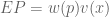
The above approaches rely on the model’s parameters (its “visceral organs”) to define complexity. But it is also possible to rely on the model’s outputs (its “behaviors”) to achieve the same task. Consider again the classification decision boundaries above. We can simply measure the spatial frequency (the “squiggliness” of the boundary) as another proxy towards complexity.
Here, then, are three possible criteria for complexity:
- Number of parameters
- Size of parameters
- Spatial frequency of decision manifold
Thus, operationalizing the definition of “complexity” is surprisingly challenging.
Mechanized Parsimony
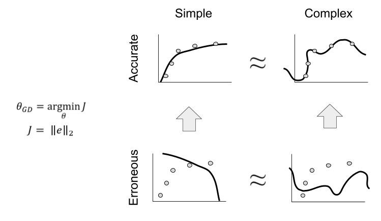
Recall our original notion of the performance-complexity quadrant. By defining our loss function exclusively in terms of the residual error, gradient descent learns to prefer accurate models (to “move upward”). Is there a way to induce leftward movement as well?
To have gradient descent respond to both criteria, we can embed them into the loss function. One simple way to accomplish this: addition.
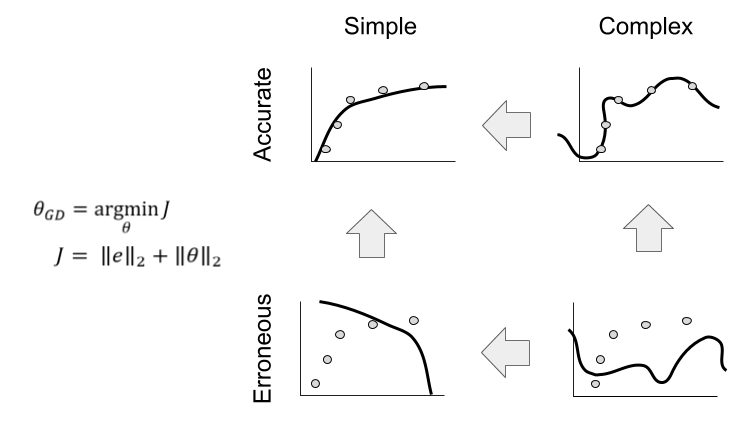
This technique is an example of regularization.
Depending on the application, sometimes the errors are much larger than the parameters or vice versa. In order to assure the right balance between these terms, people usually add a hyperparameter to the regularized loss function

A Geometric Interpretation
Recall Einstein’s insight that gravity is curvature of spacetime. You can envision such curvature as a ball pulling on a sheet. Here is the gravity well of bodies of the solar system:
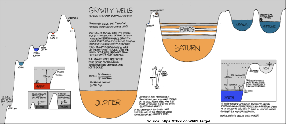
Every mass pulls on every other mass! Despite the appearance of the above, Earth does “pull on” Saturn.
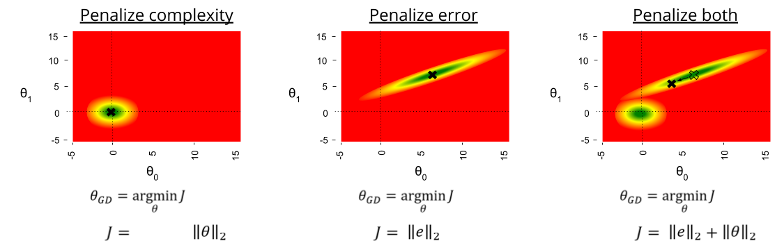
The unregularized cost function we saw last time creates a convex loss function, which we’ll interpret as a gravity well centered around parameters of best fit. If we replace J with a function that only penalizes complexity, a corresponding gravity well appears, centered around parameters of zero size.
If we keep both terms, we see the loss surface now has two enmeshed gravity wells. If scaled appropriately, the “zero attractor” will pull the most performant solution (here 

More on L1 vs L2
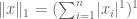
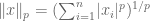
Previously, I introduced the L1 norm aka mean average error MAE
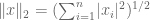
Another loss function is the L2 norm aka root mean squared error RMSE
The L1 and L2 norms respectively correspond to Euclidean vs Manhattan distance (roughly, plane vs car travel):
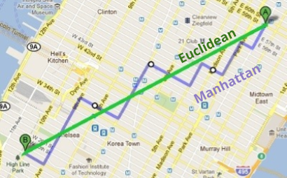
One useful way to view norms is by their isosurface. If you can travel in any direction for a finite amount of time, the isosurface is the frontier you might sketch.
The L2 isosurface is a circle. The L1 isosurface is a diamond.
- If you don’t change direction, you can travel the “normal” L2 distance.
- If you do change direction, your travel becomes inefficient (since “diagonal” travel along the hypotenuse is forbidden).
The Lp Norm as Superellipse
Consider again the formulae for the L1 and L2 norm. We can generalize these as special cases of the Lp norm:
Here are isosurfaces of six exemplars of this norm family:
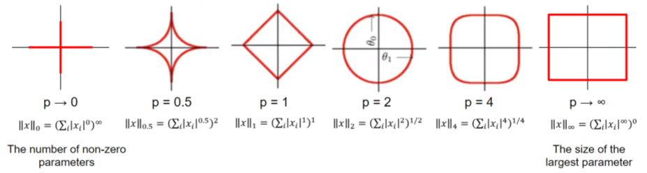
On inspection, the above image looks like a square that’s inflating with increasing p. In fact, the Lp norm generates a superellipse.
As an aside, note that the boundaries of the Lp norm family operationalize complexity rather “intuitively”. For the L0 norm, complexity is the number of non-zero parameters. For the Linf norm, complexity is the size of the largest parameter.
Lasso vs Ridge Regression
Why the detour into geometry?
Well, so far, we’ve expressed regularization as 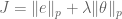
Here are two options for the residual norm:
: sensitive to outliers, but a stable solution
: robust to outlier, but an unstable solution
The instability of
That leaves us with two remaining choices:
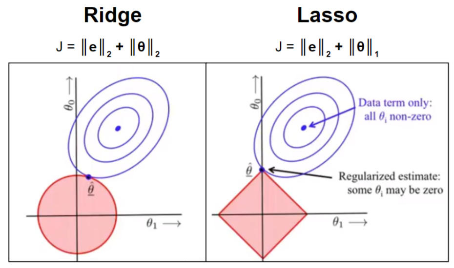
- Ridge Regression:
: computationally inefficient, but sparse output.
- Lasso Regression:
: computationally efficient, non-sparse output
What does sparse output mean? For a given model type, say 


Geometry to the rescue!
In ridge regression, both gravity wells have convex isosurfaces. Their compromises are reached anywhere in the loss surface. In lasso regression, the diamond-shaped complexity isosurface tends to push compromises towards axes where 
Both Ridge and Lasso regression are used in practice. The details of your application should influence your choice. I’ll also note in passing that “compromise algorithms” like Elastic Net exist, that tries to capture the best parts of either algorithm.
Takeaways
I hope you enjoyed this whirlwind tour of regularization. For a more detailed look at ridge vs lasso, I recommend reading this.
Until next time.


 . T
. T

 denote how many variables we admit in our context. A
  . Then the size of our CPT is
  , because we must take our original variable into account. Thus an


 . And it is true that “this” occurs only once in our toy corpus above. But out of two sentences, “this” leads half of them. We can express this fact by adding a special START token into our vocabulary.
 , because we have no instances of this two-word sequence in our toy corpus. But this causes our language model to fail catastrophically: the sentence is deemed impossible (0% probability).
 events. You’ll notice echoes of the
 -gram is not likely to occur in
  -gram model. For example, it is very possible that the phrase “dancing were thought” hasn’t been seen before.
 , we want to produce the English sentence
  such that
  .
.  , there are
  possible two-word sentences. For sentences of length
  , our time complexity of our brute force algorithm is
  .
.  : Jane is visiting Africa in September
 : Jane is going to Africa in September
 : In September, Jane went to Africa
  is the best (most probable) translation. We would like greedy search to recover it.
 , then the next word generated is
  . However, it is not difficult to contemplate
  , since the word “going” is used so much more frequently in everyday conversation. These problems of local optima happen surprisingly often.


![P[a \leq X \leq b] = \int f_X(x) dx](https://s0.wp.com/latex.php?latex=P%5Ba+%5Cleq+X+%5Cleq+b%5D+%3D+%5Cint+f_X%28x%29+dx&bg=ffffff&fg=555555&s=1&c=20201002)


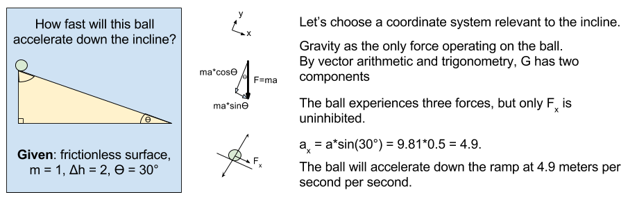

 meters per second
  m/s). However, recall the classical definitions of kinetic and potential (gravitational) energy, which are
  and
and  .
.
![m[(0 + 2g) - (\frac{ \sqrt{(4g)^2} }{2})] + 0 = m[2g - 2g] = 0](https://s0.wp.com/latex.php?latex=m%5B%280+%2B+2g%29+-+%28%5Cfrac%7B+%5Csqrt%7B%284g%29%5E2%7D+%7D%7B2%7D%29%5D+%2B+0+%3D+m%5B2g+-+2g%5D+%3D+0&bg=ffffff&fg=555555&s=0&c=20201002)
 ? Because it is experiencing a force.
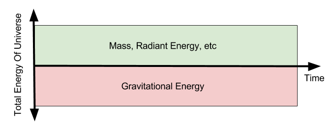


 either
  or
or  or
or 
 if
if  then
then 
 then
then  s.t.
s.t.  iff
iff 
 over
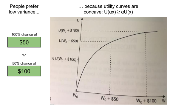
over  , mixing both with the same third lottery
  in the same proportion α must not reverse that preference—adding identical “padding” is irrelevant to the choice.


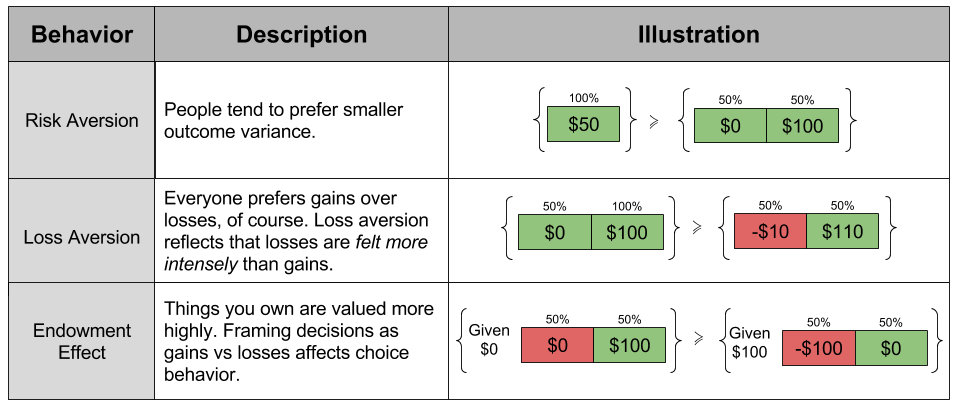
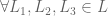
 concavity to explain risk aversion? Prospect theory takes this approach yet further, and seeks to explain all of the above behaviors using a more complex shape
 represent our updated notion of utility. We can define expected prospect
  of a function as probability multiplied by the value function

 :
:
 , captures the status quo. Thus, the reference point allows us to differentiate gains and losses, thereby producing the endowment effect.

 has the following shape:


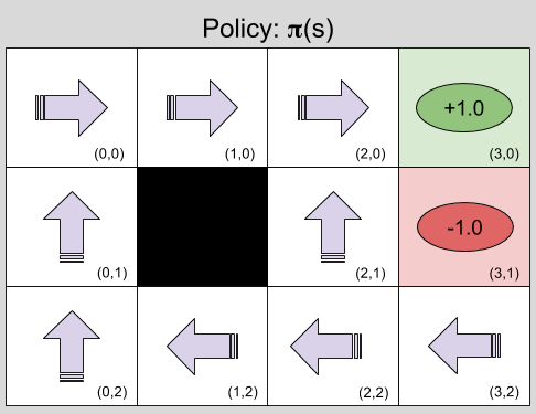


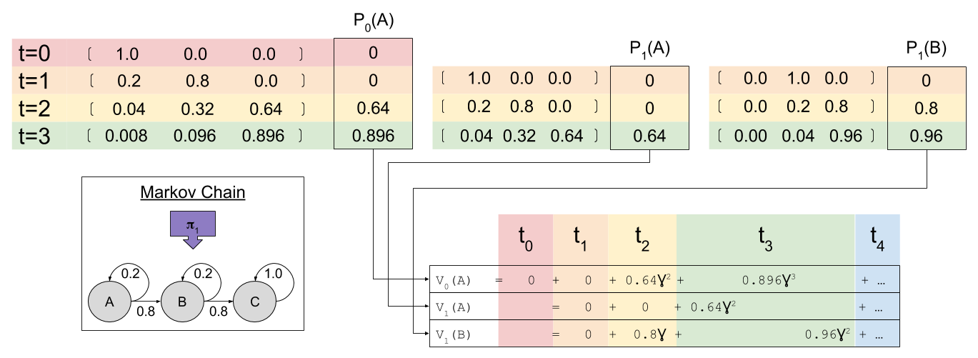
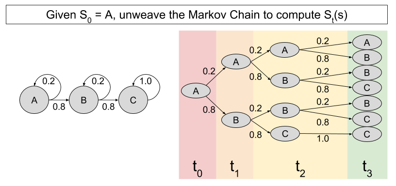
 , where
  is the state being considered at the next time step.


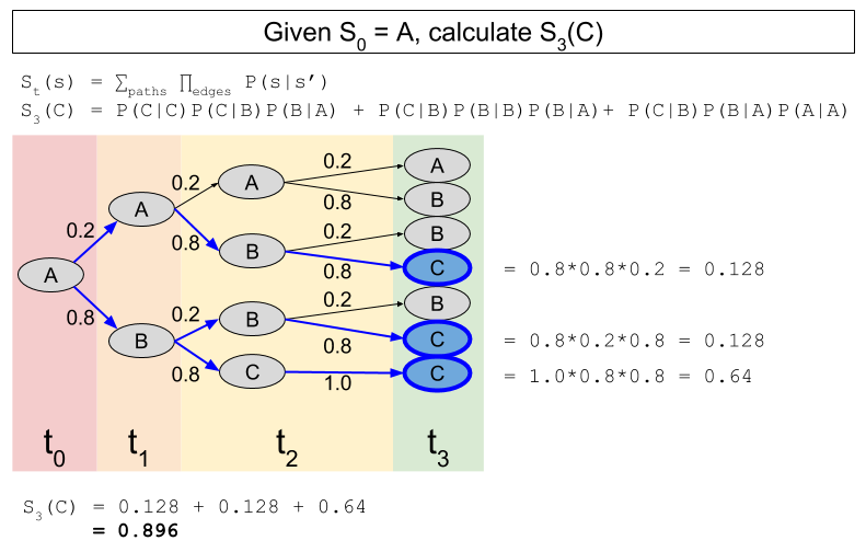
 :
:
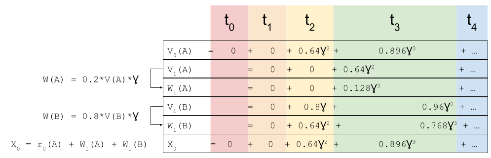
 look familiar? That’s because it equals
  ! In this way, we have a way of equating a valuation at t=0 and t=1. This property is known as intertemporal consistency.
 . Let’