An Introduction To Natural Selection

August 5, 2015March 6, 2018kevinbinz Leave a comment

Part Of: Demystifying Life sequence
Followup To: Population Genetics
Content Summary: 1400 words, 14 min read

How Natural Selection Works

Consider the following process:

Organisms pass along traits to their offspring.
Organisms vary. These random but small variations trickle through the generations.
Occasionally, the offspring of some individual will vary in a way that gives them an advantage.
On average, such individuals will survive and reproduce more successfully.

This is how favorable variations come to accumulate in populations.

Let’s plug in a concrete example. Consider a population of grizzly bears that has recently migrated to the Arctic.

Occasionally, the offspring of some grizzly bear will have a fur color mutation that renders their fur white.
This descendent will on average survive and reproduce more successfully.

Over time, we would expect increasing numbers of such bears to possess white fur.

Biological Fitness Is Height

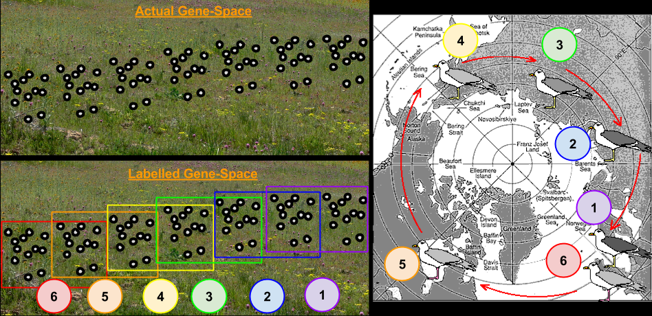
The above process is straightforward enough, but it lacks a rigorous mathematical basis. In the 1940s, the Modern Evolutionary Synthesis enriched natural selection by connecting it to population genetics, and its metaphor of Gene-Space. Recall what we mean by such a landscape:

A Genotype Is A Location.
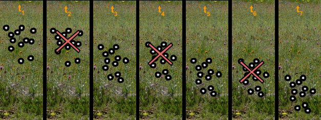
Organisms Are Unmoving Points
Birth Is Point Creation, Death Is Point Erasure
Genome Differences Are Distances

Onto this topography, we identified the following features:

A Species Is A Cluster Of Points
Species Are Vehicles
Genetic Drift is Random Travel.

In order to understand how natural selection enriches this metaphor, we must define “advantage”. Let biological fitness refer to how how many fertile offspring an individual organism leaves behind. An elephant with eight grandchildren is more fit than her neighbor with two grandchildren.

Every organism achieves one particular level of biological fitness. Fitness denotes how well-suited an organism is to its environment. Being a measure of organism-environment harmony, we can view fitness as defined for every genotype. Since we can define some number for every point in gene-space, we have license to introduce the following identification:

Biological Fitness Is Height

Here is one possible fitness landscape (image credit Bjørn Østman).

We can imagine millions of alien worlds, each with its own fitness landscape. What is the contours of Earth’s?

Let me gesture at three facts of our fitness landscape, to be elaborated next time:

The total volume of fitness is constrained by the sun. This is hinted at by the ecological notion of carrying capacity.
Fitness volume can be forcibly taken from one area of the landscape to another. This is the meaning of predation.
Since most mutations are harmless, the landscape is flat in most directions. Most non-neutral mutations are negative, but some are positive (example).

Natural Selection As Mountain Climbing

A species is a cluster of points. Biological fitness is height. What happens when a species resides on a slope?

The organisms uphill will produce comparatively more copies of themselves than those downhill. Child points that would have been evenly distributed now move preferentially uphill. Child points continue appearing more frequently uphill. This is locomotion: a slithering, amoeba-like process of genotype improvement.

We have thus arrived at a new identification:

Natural Selection Is Uphill Locomotion

As you can see, natural selection explains how species gradually become better suited to their environment. It is a non-random process: genetic movement is in a single direction.

Consider: ancestral species of the camel family originated in the American Southwest millions of years ago, where they evolved a number of adaptations to wind-blown deserts and other unfavorable environments, including a long neck and long legs. Numerous other special designs emerged in the course of time: double rows of protective eyelashes, hairy ear openings, the ability to close the nostrils, a keen sense of sight and smell, humps for storing fat, a protective coat of long and coarse hair (different from the soft undercoat known as “camel hair”), and remarkable abilities to take in water (up to 100 liters at a time) and do without it (up to 17 days).

Moles, on the other hand, evolved for burrowing in the earth in search of earthworms and other food sources inaccessible to most animals. A number of specialized adaptations evolved, but often in directions opposite to those of the camel: round bodies, short legs, a flat pointed head, broad claws on the forefeet for digging. In addition, most moles are blind and hard of hearing.

The mechanism behind these adaptations is selection, because each results in an increase in fitness, with one exception. Loss of sight and hearing in moles is not an example of natural selection, but of genetic drift: blindness wouldn’t confer any advantages underground, but arguably neither would eyesight.

Microbiologists in my audience might recognize a strong analogy with bacterial locomotion. Most bacteria have two modes of movement: directed movement (chemotaxis) when its chemical sensors detect food, and a random walk when no such signal is present. This corresponds with natural selection and genetic drift, respectively.

Consequences Of Optimization Algorithms

Computer scientists in my audience might note a strong analogy to gradient descent, a kind of algorithm. In fact, there is a precise sense in which natural selection is an optimization algorithm. In fact, computer scientists have used this insight to design powerful evolutionary algorithms that spawn not one program, but thousands of programs, rewarding those with a comparative advantage. Evolutionary algorithms have proven an extremely fertile discipline in problem spaces with high dimensionality. Consider, for example, recent advances in evolvable hardware:

As predicted, the principle of natural selection could successfully produce specialized circuits using a fraction of the resources a human would have required. And no one had the foggiest notion how it worked. Dr. Thompson peered inside his perfect offspring to gain insight into its methods, but what he found inside was baffling. The plucky chip was utilizing only thirty-seven of its one hundred logic gates, and most of them were arranged in a curious collection of feedback loops. Five individual logic cells were functionally disconnected from the rest— with no pathways that would allow them to influence the output— yet when the researcher disabled any one of them the chip lost its ability to discriminate the tones…

It seems that evolution had not merely selected the best code for the task, it had also advocated those programs which took advantage of the electromagnetic quirks of that specific microchip environment. The five separate logic cells were clearly crucial to the chip’s operation, but they were interacting with the main circuitry through some unorthodox method— most likely via the subtle magnetic fields that are created when electrons flow through circuitry, an effect known as magnetic flux. There was also evidence that the circuit was not relying solely on the transistors’ absolute ON and OFF positions like a typical chip; it was capitalizing upon analogue shades of gray along with the digital black and white.

In gradient descent, there is a distinction between global optima and local optima. Despite the existence of an objectively superior solution, the algorithm cannot get there due to its fixation with local ascent.

This distinction also features strongly in nature. Consider again our example of camels and moles:

Given such a stunning variety of specialized differences between the camel and the mole, it is curious that the structure of their necks remains basically the same. Surely the camel could do with more vertebrae and flex in foraging through the coarse and thorny plants that compose its standard fare, whereas moles could just as surely do with fewer vertebrae and less flex. What is almost as sure, however, is that there is substantial cost in restructuring the neck’s nerve network to conform to a greater or fewer number of vertebrae, particularly in rerouting spinal nerves which innervate different aspects of the body.

Here we see natural selection as a “tinkerer”; unable to completely throw away old solutions, but instead perpetually laboring to improve its current designs.

Takeaways

In the landscape of all possible genomes, we can encode comparative advantages as differences in height.
Well-adapted organisms are better at replicating their genes (in other words, none of your ancestors were childless).
Viewed in the lens of population genetics, natural selection becomes a kind of uphill locomotion.
When view computationally, natural selection reveals itself to be an optimization algorithm.
Natural solution can outmatch human intelligence, but it is also a “tinkerer”; unable to start from scratch.

An Introduction To Population Genetics

August 2, 2015March 23, 2017kevinbinz Leave a comment

Part Of: Demystifying Life sequence
Content Summary: 1200 words, 12 min read

Central Thesis Of Molecular Biology

In every cell of your body, there exist molecules called deoxyribonucleic acid. Such cells come in four flavors and (due to their atomic shape) tend to pair up and create long strings. These strings become very long, over two inches when held end-to-end (but of course, they fold up dramatically so each can comfortably inhabit a single cell). Since your cells have about 46 inches worth (six billion molecules), each cell contains twenty-three unique strings. They look like this:

Let us refer to these strings as chromosomes, and to all of them collectively as the human genome. Finally, since typing “deoxyribonucleic acid” is fairly onerous, we will use the acronym DNA.

In 1956, Francis Crick presented his Central Thesis Of Molecular Biology, which describes how the causal chain DNA → RNA → amino acids → protein ultimately motivates every trait of every living organism. A gene is a sequence of DNA that encodes a protein. A genotype (some animal’s unique DNA) explains phenotype (that animal’s unique traits). Genotype-phenotype maps (GP-maps) turn out to be very important in what follows.

Duplication vs. Mutation

Every time a cell duplicates itself (mitosis), its DNA is copied into the new cell. If every cell contains exactly the same code, how can they be different? The basic explanation of cellular differentiation involves feedback loops in the genetic causal chain (collectively named the Gene Regulatory Network). When a lung cell is duplicated, for example, it inherits not just the entire genome, but also proteins for activating lung genes and deactivating other code.

Germ cells are created by a different process entirely. Instead of genome duplication (mitosis), germ cells inherit what is essentially half a genome, in a process known as meiosis. Here’s how these two processes work:

Recall that deoxyribonucleic acid is a collection of atoms. Replicating such a fragile object is imperfect. There are many kinds of ways the process can go wrong; for example:

Replacement Mutation (e.g., AGTC → AATC)
Duplication Mutation (e.g., AGTC → AGGTC)
Insertion Mutation (e.g., AGTC → AGATC)

How many mutations do you have? While you can always get your DNA sequenced to find out, the answer for most people is about sixty.

The Landscape Of Gene-Space

Consider all animals whose genome is three molecules long. How many genetically unique kinds of these animals are there? Recall there are four kinds of DNA: cytosine (C), guanine (G), adenine (A), or thymine (T). We can use the following formula:

$|Permutations| = |Possibilities|^{|Slots|}$

Here we have 3^4 = 81 possible genotypes in this particular gene-space. To visualize this, imagine a 4-sided Rubik’s Cube: each dimension is a slot, each cube a particular genotype in the space.

But humans have approximately three billion base pairs; the size of a realistic gene-space is almost incomprehensibly large (4^3,000,000,000), far exceeding the number of atoms in the universe. Reasoning about 3D cubes is easy, reasoning about 3,000,000,000-D hypercubes is a bit harder. So we employ dimension reduction to aid comprehension. If you laid all 4^3,000,000,000 numbers out on a two dimensional matrix, each cell would be so tiny that the surface would appear continuous. We have arrived at our first metaphor identification:

A Genotype Is A Location

We can summarize our discussion of mitosis, meiosis, and mutation as follows:

An Organism Is A Stationary Point
Birth Is Point Creation, Death Is Point Erasure.

Finally, let us explore the concept of genetic distance. From our toy gene-space, let me take seven nodes and draw lines indicating valid replacement mutations between them.

The key observation is that distances vary. Many nodes are connected via one mutation, but the minimum distance from top (ATG) to bottom (CCC) is three mutations. In other words:

Varying Genome Differences Are Varying Distances

Our gene-space landscape, then, looks something like this:

Species Are Clusters

What is a species? After all, there is no encoding of the word “jaguar” in the jaguar genome. Rather, members of a species share more genetic similarities to one another than other organisms. In terms of our metaphor:

A Species Is A Cluster Of Points

In the above landscape, we might have two species. But there are many ways to cluster data. Consider these competing definitions:

Which clustering approach is correct? It depends on the scale of our axes:

If we chose Granular but are too “zoomed in”, we have accidentally defined four new species of Shih Tzu.
If we chose Course but are too “zoomed out”, we have accidentally defined Mammal as its own species.

The point is that scale matters, and we should define species on a scale that makes good biological sense. The most popular scale is that defined by successful interbreeding (i.e., produce fertile offspring). For greater distances (large genetic dissimilarity), such interbreeding is impossible. We therefore constrain the size of our specie clusters by maximum interbreeding distance.

The approach just outlined is the one in use today. However, any man-made criteria for categorizing reality has its stretch points. For example, consider ring species.

Consider the Larus gulls’ populations in the above image. These gulls habitats form a ring around the North Pole, not normally crossed by individual gulls. The European herring gull {6} can hybridize with the American herring gull {5}, which can hybridize with the East Siberian herring gull {4} which can hybridize with Heuglin’s gull {3}, which can hybridize with the Siberian lesser black-backed gull {2}, which can hybridize with the lesser black-backed gulls {1}. However, the lesser black-backed gulls {1} and herring gulls {6} are sufficiently different that they do not normally hybridize.

Genetic Drift Is Random Travel

Landscapes without movement aren’t very interesting. With our brand-new concept as Species As Clusters, let’s see if we can make sense of travel.

Consider the phenomenon of population bottleneck. Many factors may contribute to population reduction (e.g., novel predators). Often, the survivors are just lucky. Descendants of the survivors tend to be more similar to them than the average genome of the original species. By this process, bottlenecks induces change in the species as a whole:

Why wouldn’t such movement cancel itself out in the long run? The reason why resides in the size of gene-space. For our genome is length two, mutations cancelling each other out would be a fairly common occurence. Would cancelling out increase or decrease on a genome of length 1,000? Surely less. How much less (a forteriori!) the case for genomes with three billion molecules. By the extreme dimensionality of gene-space, then, we are witness to non-cancellative genetic movement!

Genetic Drift Is (Random) Travel.

Importantly, it is not the individuals that travel (modify their genomes), but the species as a whole.

Species Are Vehicles.

Viewing the species itself as actor, rather than the individual, is an important paradigm shift of population genetics.

Takeaways

In this post, I introduced the following metaphor:

A Genotype Is A Location.
Organisms Are Unmoving Points
Birth Is Point Creation, Death Is Point Erasure
Genome Differences Are Distances

We then strengthened our metaphor with the following considerations:

A Species Is A Cluster Of Points
Species Are Vehicles
Genetic Drift is (Random) Travel.

We are left with the image of specie vehicles clumsily moving around gene-space. But genetic drift is not the only mechanism by which species navigate gene-space. In our next post, we explore a more sophisticated property of living things.

An Introduction To Category Theory [Part One]

July 16, 2015July 17, 2015kevinbinz Leave a comment

What’s So Important About Graphs?

Of all the conceptual devices in my toolkit, hyperpoints and graphs are employed the most frequently. I have explained hyperpoints previously; let me today explain What’s So Important About Graphs?

Human beings tend to divide the world into states versus actions. This metaphor is so deeply ingrained in our psyche that it tends to be taken for granted. Graphs are important because they visualize this state-action dichotomy: states are dots, actions are lines.

Put crudely, graphs are little more than connect-the-dots drawings. Now, dear reader, perhaps you do not yet regularly contemplate connect-the-dots in your daily life. Let me paint some examples to whet your appetite.

Maps are graphs. Locations are nodes, paths are the edges that connect them.
Academic citations are a graph. Papers are nodes, citations are the edges that connect them.
Facebook is a graph. People are nodes, friendships are the edges that connect them.
Concept-space is a graph. Propositions are nodes, inference are the edges that connect them.
Causality is a graph. Effects are nodes, causes are the edges that connect them.
Brains are graphs. Neurons are nodes, axons are the edges that connect them.

The above examples are rather diverse, yet we can reason about them within a single framework. This is what it means to consolidate knowledge.

Graph Theory: Applications & Limitations

It turns out that a considerable amount of literature lurks beneath each of our examples. Let’s review the highlights.

Once upon a time, Karl Popper argued that a scientific theory is only as strong as it is vulnerable to falsification. General relativity made the crazy prediction of gravitational lensing which was only later confirmed experimentally. One reason to call astrology “pseudoscience” is in its reluctance to produce such a vulnerable prediction.

But simple falsification doesn’t fully describe science: healthy theories can survive certain kinds of refutations. How? W. V. O. Quine appealed to the fact that beliefs cannot be evaluated in isolation; we must instead view scientific theories as a “web of belief”. And this web can be interpreted graphically! Armed with this interpretation, one can successfully evaluate philosophical arguments involving Quine’s doctrine (called confirmation holism) based on technical constraints on graphical algorithms.

The modern incarnation of confirmation holism occurs when you replace beliefs with degrees-of-belief. These probabilistic graphical models are powerful enough to formally describe belief propagation.

But even probabilistic graphical models don’t fully describe cognition: humans possess several memory systems. Our procedural memory (“muscle memory”) is a graph of belief, and our episodic memory (“story memory”) is a separate graph of belief.

How to merge two different graphs? Graph theory cannot compose graphs horizontally.

Switching gears to two other examples:

The formal name for brains-are-graphs is neural networks. They are the lifeblood of computational neuroscientists.
The formal name for Facebook-is-a-graph is social networks. They are vital to the research of sociologists.

How might a neuroscientist talk to a sociologist? One’s network represents the mental life of a person; the other, the aggregate lives of many people. We want to say is that every node in a social graph contains an entire neural graph.

How to nest graphs-within-graphs? Graph theory cannot compose graphs vertically.

The Categorical Landscape

What are categories? For us, categories generalize graphs.

A directed graph can be expressed G = (V, E); that is, it contains a set of nodes, and a set of edges between those nodes.

A small category C = (O, M); that is, it contains a set of objects, and a set of morphisms between those objects.

Categories endow graphs with additional structure.

Category Theory require the notion of self-loops: actions that result in no change.
In Graph Theory, there is a notion of paths from one node to another. Category Theory promote every path into its very own morphism.
Category Theory formalizes the notion of context: objects and morphisms live within a common environment; this context is called a “category”.

As an aside, directed graphs require only one edge between graphs, and no self-loops. We could tighten the analogy yet further by comparing categories to quivers (directed graphs that don’t forbid parallel edges and self-loops).

But enough technicalities. Time to meet to your first category! In honor of category theory’s mathematical background, allow me to introduce Set. In Set, objects are sets, and morphisms are functions. Here is one small corner of the category:
Self-loops 1_A, 1_B, and 1_C change nothing; they are special kind of self-loops called identity morphisms. Since such things exist on every node, we will henceforth consider their existence implicit.

Recall our requirement that every path has a morphism. The above example contains three paths:

π₁ = A → B
π₂ = B → C
π₃ = A → B → C

The first two paths are claimed by f and g, respectively, but the third is unaffiliated. For this to qualify as a category, we must construct for it a new morphism. How? We create h : A → C via function composition:

h(x) = g(f(x)) = [f(x)]-1 = 2x-1.

We also require morphism composition to be associative. Another example should make this clear:

Besides g(f(x)), we can also write function composition as f●g (“f then g”). In the above, we have:

i(x) = f●g
j(x) = g●h
k(x) = f●g●h

With this notation, we express our requirement for morphism associativity as

k = (f●g)●h = f●(g●h).
That is, k = i●h = f●j.
That is, “you can move from A to D by travelling either along i-then-h, or along f-then-j”.

Harden The Definition

Let me be precise. Categories contain two types of data:

A set of objects O.
A set of morphisms M such that m : A → B

The set of morphisms is required to contain the following two sets:

A set of identity morphisms 1 such that 1_A : A → A
A set of composition morphisms such that for every f : A → B and g: B → C, there is a morphism h: A → C.

The set of morphisms is required to respect the following two rules:

Identity: composing a morphism with an identity does nothing. f●1 = f = 1●f
Associativity: the order in which you compose functions doesn’t matter. (f●g)●h = f●(g●h)

Connecting To Group Theory

Recall that groups define axioms governing set operations. A group might choose to accept or reject any of the following axioms:

Closure
Associativity
Identity Element
Inverse Element
Associativity

We can now better appreciate our taxonomy from An Introduction To Group Theory:

Take a second to locate the Category group. Do you see how its two axioms align with our previous definition of a category?

Notice that in group theory, categories are kind of a degenerate monoid. Why have we removed the requirement for closure?

We can answer this question by considering the category SomeMonoid? It turns out that this category has only one object (with each of its member elements as self-loops). This is the categorical consequence of closure. We do not require closure in our category theory because we want license to consider categories with a multitude of objects.

Takeaways

In this article, I introduced graphs, and used human memory and social vs. neural networks to motivate two limitations of graph theory:

How to merge two different graphs? Graph theory cannot compose graphs horizontally.

How to nest graphs-within-graphs? Graph theory cannot compose graphs vertically.

I then introduced you to Category Theory, showing how it both generalizes graph theory and connects to abstract algebra.

In the final half of this introduction, I will discharge my above two commitments. Specifically, next time I will show how:

The concept of functor permits horizontal composition of categories.

The distinction between “inside” and “outside” views facilitates vertical composition of categories.

An Introduction To Structural Realism

July 7, 2015March 21, 2017kevinbinz Leave a comment

Part Of: Philosophy of Science sequence
Content Summary: 900 words, 9 min read

Does science describe the world? Let me frame this foray into philosophy of science as a dialectic.

The Exchange

It is a brisk spring evening, just before sunset. Achilles and the Tortoise are taking their ritualized evening stroll down a winding country road. Their discussions vary wildly, but typically center around some current events or some random bit of science news.

Achilles comments out of the blue: “Tortoise, I can’t help but notice that you seem to place too much weight in scientific claims.”
“Do you really doubt the existence of the electron?” the Tortoise counters. “I mean, if particle physics got that wrong, then how could it wield such predictive power?”
Achilles’ pace slows, as he puzzles over the Tortoise’s reply. “But doesn’t it strike you as arrogant to believe we were lucky enough to be born in an age where science got it right? I would probably credit my skepticism to my reading of scientific history, at watching long lines of scientific theories crumble and fall.”
Tortoise replies: “Achilles, I have a slogan I like to tell people, to explain my way of thinking. When people thought the earth was flat, they were wrong. When people thought the earth was spherical, they were wrong. But if you really think that thinking the earth is spherical is just as wrong as thinking the earth is flat, then your view is wronger than both of them put together.”
Tortoise continues: “My point is simply that your binary notion of truth must become more subtle. It seems better to say that modern theories (such as general relativity) approximate older theories (like Newtonian mechanics).”

Now, in case you haven’t heard these arguments before, Achilles is Thomas Kuhn and Tortoise is Isaac Asimov. I have found the appeal to approximation compelling, and so (I submit) do most scientists. However, here is the depth at which most people stop. Let us instead swim further… let us listen more carefully to Achilles.

Achilles gathers his thoughts. “When you read your textbooks, Tortoise, how many hours do you spend perusing the history section?”
“Not many, Achilles.” The Tortoise seems neither apologetic nor proud of this fact. “While Tortoises do in fact live for 200 years, my time is still finite. I’d rather let my mind reside near the state of the art.”
“Of course learning about history is not for everyone, Tortoise… but I have. Consider what it would feel like to read science textbooks from my eyes. Naturally enough, these texts are written by the victors of scientific disputes… but their history sections without fail do violence to the actual thinking of their predecessors.” Achilles’ speech is picking up speed. “Tortoise, if you study history like I do, your nose would smell propaganda, as mine does.”
Achilles drives his point home: “Shouldn’t this stench give you pause, Tortoise? Your claim about scientific revolutions approximating their predecessors strikes you as intuitive, but do historians concur? In fact, you stand at odd with the facts of scientific revolutions. General relativity was not conceived as a generalization of classical mechanics. What relativistic concept does the Newtonian concept of simultaneity ‘approximate’? It does not! Consider also the ether. It was not approximated, it was trashed! Your notion of approximation seems misguided, my friend.”

This is the Kuhnian critique of scientific realism. Most philosophers consider the strongest reply to go as follows:

Startled at his inability to defend his vague notions, Tortoise spends the next several months studying scientific histories, and trying to improve his theory of approximation. Spring turns into summer… but then one day, Tortoise feels ready to return to this topic:

“Achilles, do you remember our conversation about scientific histories?”
“Of course I do, Tortoise!”
“Well, It seems to me that you’ve put your finger on something important. I’ve spent time poring over memoirs of past intellectual giants as you have, and I definitely now see what you mean by the ‘smell of propaganda’. But Achilles, I think I’ve noticed something else, something important”.
Tortoise continues: “When I look at the debates between competing theories, my cherished notion of approximation cannot be resuscitated. But! When I compare the equations of new theories to the ones they replace, I do see an approximation. For example, I cannot recover the Newtonian dogma of flat three-dimensional space, but if I assume the speed of light is infinite, I can recover the Newtonian equation of gravity directly from general relativity.”
Tortoise concludes: “Achilles, it seems to me that the only continuity in science is in its laws. I will no longer claim to know that electrons are real, or that spacetime is curved. Concepts may not refer. It is only the relationship between concepts, the formal structure of a mature theory, that lasts”.

Condensing The Argument

The above conversation is based on (Worrall, 1989) Structural Realism: The Best Of Both Worlds?. We can compress the above as follows:

Realists advance the no-miracles argument: the predictive power of science seems too implausible unless its theories somehow refer to reality.
Anti-realists counter with pessimistic meta-induction: previously successful theories have been discarded; who are we to say that our current theories won’t meet the same fate.
The approximation hypothesis is where these two arguments connect meaningfully: isn’t it more accurate to call older theories approximations rather than worthless?
It is notoriously difficult to describe what “approximation” means.
Some realists have conceded that scientific narratives tend to fail, but produce compelling evidence that scientific equations tend to persist. This position is known as structural realism (where formulae structure means more than the meaning of the variables).

An Introduction To Prisoner’s Dilemma

June 5, 2015March 22, 2017kevinbinz Leave a comment

Part Of: Algorithmic Game Theory sequence
Content Summary: 600 words, 6 min read

Setting The Stage

The Prisoner’s Dilemma is a thought experiment central to game theory. It goes like this:

Two members of a criminal gang are arrested and imprisoned. Each prisoner is in solitary confinement with no means of speaking to or exchanging messages with the other. The police admit they don’t have enough evidence to convict the pair on the principal charge. They plan to sentence both to a year in prison on a lesser charge.

Simultaneously, the police offer each prisoner a Faustian bargain. Each prisoner is given the opportunity either to betray the other, by testifying that the other committed the crime, or to cooperate with the other by remaining silent:

If A and B both betray the other, each of them serves 2 years in prison

If A betrays B but B remains silent, A will be set free and B will serve 3 years in prison (and vice versa)

If A and B both remain silent, both of them will only serve 1 year in prison (on the lesser charge)

Do you “get” the dilemma? Both prisoners do better if they each cooperate with one another. But they are taken to separate rooms, where the decisions of the other are no longer visible. The question evolving towards one of trust…

This parable can be drawn in strategy-space:

Strategic Dominance

Consider Person A’s perspective:

One line of analysis might run as follows:

If the other person cooperates (top rectangle), Player A would do better defecting (rightmost cell).
If the other person defects (bottom rectangle), Player A would do better defecting (rightmost cell).

Thus, no matter what B’s choice, defection leads to a superior result. Let us call this strategic dominance.

Person B’s perspective, in the below figure, is analogous:

If the other person cooperates (left rectangle), Player A would do better defecting (bottom cell).
If the other person defects (right rectangle), Player A would do better defecting (bottom cell).

Thus, the strategically dominant outcome is Defect-Defect, or (D, D).

Pareto Optimality

If the prisoners could coordinate their responses, would they select (D,D)? Surely not.

How might we express our distaste for mutual defection rigorously? One option would be to notice that (C, C) is preferred by both players. Is there anything better than mutual cooperation, in this sense? No.

Let us call the movement from (D,D) to (C,C) a Pareto improvement, and the outcome (C,C) Pareto optimal (that is, no one player’s utility can be improved without harming that of another).

It turns out that (C,D) and (D, C) are also Pareto optimal. If we map all outcomes in utility-space, we notice that Pareto optimal outcomes comprise a “fence” (also called a Pareto frontier).

The crisis of the Prisoner’s Dilemma can be put as follows: (D, D) doesn’t reside on the Pareto frontier. More generally: strategically-dominant outcomes need not reside on the Pareto frontier.

While there are other, more granular, ways to express “good outcomes”, the Pareto frontier is a useful way to think about the utility landscape.

Let me close with an observation I wish I had encountered sooner: utility-space does not exist a priori. It is an artifact of causal processes. One might even question the ethics of artificially inducing “Prisoner’s Dilemma” landscapes, given their penchant for provoking antisocial behaviors.

Takeaways

A strategy is called dominant when it always outperforms alternatives, irrespective of competitor behavior.
Pareto optimal outcomes are those for which there is no “pain-free” way to improve the outcome of any participant. All such outcomes comprise the Pareto frontier.
The Prisoner’s Dilemma illustrates that strategically-dominant outcomes need not reside on the Pareto frontier, or more informally, that acting in one’s self-interest can lead to situations where everyone loses.

An Introduction To Newcomb’s Paradox

November 2, 2014March 27, 2017kevinbinz Leave a comment

Part Of: Algorithmic Game Theory sequence
Related To: An Introduction To Prisoner’s Dilemma
Content Summary: 1000 words, 10 min read

The Paradox

Newcomb’s Paradox is a thought experiment popularized by philosophy superstar Robert Nozick in 1969, with important implications for decision theory:

A superintelligence from another galaxy, whom we shall call Omega, comes to Earth and sets about playing a strange little game. In this game, Omega selects a human being, sets down two boxes in front of them, and flies away.

Box A is transparent and contains a thousand dollars.

Box B is opaque, and contains either a million dollars, or nothing.

You can take both boxes, or take only box B.

And the twist is that Omega has put a million dollars in box B iff Omega has predicted that you will take only box B.

Omega has been correct on each of 100 observed occasions so far – everyone who took both boxes has found box B empty and received only a thousand dollars; everyone who took only box B has found B containing a million dollars. (We assume that box A vanishes in a puff of smoke if you take only box B; no one else can take box A afterward.)

Before you make your choice, Omega has flown off and moved on to its next game. Box B is already empty or already full.

Omega drops two boxes on the ground in front of you and flies off.

Do you take both boxes, or only box B?

Well, what’s your answer? 🙂 Seriously, make up your mind before proceeding. Do you take one box, or two?

Robert Nozick once remarked that:

To almost everyone it is perfectly clear and obvious what should be done. The difficulty is that people seem to divide almost evenly on the problem, with large numbers thinking that the opposing half is just being silly.

The disagreement seems to stem from the contradiction of two strong intuitions: one “altruistic” intuition in favor of 1-box, the other 2-box intuition is more “selfish”. They are, respectively:

Expectation Intuition: Take the action with the greater expected outcome.
Maximization Intuition: Take the action which, given the current state of the world, guarantees you a better outcome than any other action.

Allow me to visualize the mechanics of this thought experiment now (note that the Predictor is a not-necessarily-omniscient version of Omega):

Still with me? 🙂 Good. Let’s see if we can use game theory to mature our view of this paradox.

Game-Theoretic Lenses

Do you remember Introduction To Prisoner’s Dilemma? At one point in that article, we decomposed the problem into a decision matrix. We can do the same thing for this paradox, too:

From the perspective of the Decider, strategic dominance here cash out our Intuition #1: the bottom row always outperforms the top row.

However, the point of making the Predictor knowledgeable is that landing in the gray cells (top-right, bottom-left) become unlikely. Let us make the size of our boxes represent the chance that they will occur.

With a Predictor of infinite accuracy, the size of the gray cells becomes zero, and now 1-Boxing suddenly dominates 2-Boxing.

With a Predictor with bounded intelligence, what follows? Might some logic be constructed to describe optimal choices in such a scenario?

A Philosophical Aside

Taken from this excellent article:

The standard philosophical conversation runs thusly:

One-boxer: “I take only box B, of course. I’d rather have a million than a thousand.”

Two-boxer: “Omega has already left. Either box B is already full or already empty. If box B is already empty, then taking both boxes nets me $1000, taking only box B nets me $0. If box B is already full, then taking both boxes nets $1,001,000, taking only box B nets $1,000,000. In either case I do better by taking both boxes, and worse by leaving a thousand dollars on the table – so I will be rational, and take both boxes.”

One-boxer: “If you’re so rational, why ain’cha rich?”

Two-boxer: “It’s not my fault Omega chooses to reward only people with irrational dispositions, but it’s already too late for me to do anything about that.”

One-boxer: “What if the reward within box B are something you could not leave behind? Would you still fall on your sword?”

Who wins, according to the experts? No consensus exists. Some relevant results, taken from a survey of professional philosophers:

Newcomb’s problem: one box or two boxes?

Accept or lean toward: two boxes 292 / 931 (31.4%)

Accept or lean toward: one box 198 / 931 (21.3%)

Don’t know 441 / 931 (47.4%)

Prediction Is Time Travel

There is a wonderfully recursive nature to Newcomb’s problem: the accuracy of the predictor stems from it modelling your decision machinery.

In this (more complete) diagram, we have the Predictor building a model of your cognitive faculties via the proxy of behavior.

As the fidelity of its model (gray image in the Predictor) improves as more information is pulled from the Decider (red arrow) the more perfect its predictive accuracy, (reduced size of the gray outcome-rectangles).

The Decider may say to herself:

Oh, if only my mind were such that the “altruistic” Expectation Intuition could win at prediction-time, but the “selfish” Maximization Intuition could win at choice-time.

Then, I would deceive the Predictor. Then, I would win $1,001,000.

But even if she possesses the ability to control her mind in this way, a perfect Predictor will learn of it. Thus, the Decider may reason:

If my changing my mind is so predictable, perhaps I might find some vehicle to change my mind based on the results of coin-flip…

What the Decider is trying to do, here, is a mechanism to corrupt the Predictor’s knowledge. How might a Predictor respond to such attacks of deterministic prediction?

Open Questions

This article represents more of an exploration, than a tour of hardened results.

Maybe I’ll produce revision #2 at some point… anyways, to my present self, the following are open questions:

How can we get clear on the relations between Newcomb’s Paradox and game theory more generally?
How might the “probability mass” lens be used to generalize this paradox to non-perfect Predictors
How might the metaphysics of retroactive causality, or at least the intuitions behind such constructs, play into the decision?
How much explanatory power does the anti-maximization principle behind 1-boxing (and the ability to precommit to such “altruistic irrationality”) say about human feelings of guilt or gratitude?
How might this subject be enriched by complexity theory, and metamathetics?
How might this subject enrich discussions of reciprical altruism and hyperbolic discounting?

Until next time.

An Introduction To Hyperbolic Discounting

September 14, 2014August 15, 2015kevinbinz Leave a comment

Part Of: [Breakdown of Will] sequence

Table Of Contents

What Is Akrasia?
Utility Curves, In 200 Words Or Less!
Choosing Marshmallows
Devil In The (Hyperbolic) Details
The Self As A Population
Takeaways

What Is Akrasia?

Do you agree or disagree with the following?

In a prosperous society, most misery is self-inflicted. We smoke, eat and drink to excess, and become addicted to drugs, gambling, credit card abuse, destructive emotional relationships, and simple procrastination, usually while attempting not to do so.

It would seem that behavior contradicting one’s own desires is, at least, a frustratingly common human experience. Aristotle called this kind of experience akrasia. Here’s the apostle Paul’s description:

I do not understand what I do. For what I want to do I do not do, but what I hate I do. (Romans 7:15)

The phenomenon of akrasia, and the entire subject of willpower generally, is controversial (a biasing attractor). Nevertheless, both its description and underlying mechanisms are empirically tractable. Let us now proceed to help Paul understand, from a cognitive perspective, the contradictions emerging from his brain.

We begin our journey with the economic concept of utility.

Utility Curves, In 200 Words Or Less!

Let utility here represent the strength with which a person desires a thing. This value may change over time. A utility curve, then, simply charts the relationship between utility and time. For example:

Let’s zoom in on this toy example, and name three temporal locations:

Let t_beginning represent the time I inform you about a future reward.
Let t_reward represent the time you receive the reward.
Let t_middle represent some intermediate time, between the above.

Consider the case when NOW = t_beginning.At that time, we see that the choice is valued at 5 “utils”.

Consider what happens as the knife edge of the present (the red line) advances. At NOW = t_middle, the utility of the choice (the strength of our preference for it) doubles:

Increasing utility curves also go by the name discounted utility, which stems from a different view of the x-axis (at the decision point looking towards the past, or setting x to be in units of time delay). Discounted utility reflect something of human psychology: given a fixed reward, other things equal, receiving it more quickly is more valuable.

This concludes our extremely complicated foray into economic theory. 😛 As you’ll see, utility curves present a nice canvas on which we can paint human decision-making.

Choosing Marshmallows

Everyday instances of akrasia tend to be rather involved. Consider the decision to maintain destructive emotional relationships: the underlying causal graph is rather difficult to parse.

Let’s simplify. Ever heard of the Stanford Marshmallow Experiment?

In these studies, a child was offered a choice between one small reward (sometimes a marshmallow) provided immediately or two small rewards if he or she waited until the tester returned (after an absence of approximately 15 minutes). In follow-up studies, the researchers found that children who were able to wait longer for the preferred rewards tended to have better life outcomes, as measured by SAT scores, educational attainment, body mass index (BMI) and other life measures.

Naming the alternatives:

SS reward: Call the immediate, one-marshmallow option the SS (smaller-sooner) reward.
LL reward: Call the delayed, two-marshmallow option the LL (larger-later) reward.

Marshmallows are simply a playful vehicle to transport concepts. Why are we tempted to reach for SS despite knowing our long-term interests lie with LL?

Here’s one representation of the above experiment (LL is the orange curve, SS is green):

Our definition of utility was very simple: a measure of preference strength. This article’s model of choice will be equally straightforward: humans always select the choice with higher utility.

The option will people select? Always the orange curve. No matter how far the knife edge of the present advances, the utility of LL always exceeds that of SS:

Shockingly, economists like to model utility curves like these with mathematical formulas, rather than Google Drawings. These utility relationships can be produced with exponential functions; let us call them exponential discount curves.

Devil In The (Hyperbolic) Details

But the above utility curves are not the only one that could be implemented in the brain. Even if we held Utility(t_beginning) and Utility(t_reward) constant, the rate at which Utility(NOW) increases may vary. Consider what happens when most of the utility obtains close to reward-time (when the utility curves form a “hockey stick”):

Let us quickly ground this alternative in a mathematical formalism. A function that fits our “hockey stick” criteria is the hyperbolic function; so we will name the above a hyperbolic discount curve.

Notice that the above “overlap” is highly significant – it indicates different choices at different times:

This is the birthplace of akrasia – the cradle of “sin nature” – where SS (smaller-sooner) rewards temporarily outweigh LL (larger-later) rewards.

The Self As A Population

Consider the story of Odysseus and the sirens:

Odysseus was curious as to what the Sirens sang to him, and so, on the advice of Circe, he had all of his sailors plug their ears with beeswax and tie him to the mast. He ordered his men to leave him tied tightly to the mast, no matter how much he would beg. When he heard their beautiful song, he ordered the sailors to untie him but they bound him tighter.

With this powerful illustration of akrasia, we are tempted to view Odysseus as two separate people. Pre-siren Odysseus is intent on sailing past the sirens, but post-siren Odysseus is desperate to approach them. We even see pre-siren Odysseus restricting the freedoms of post-siren Odysseus…

How can identity be divided against itself? This becomes possible if we are, in part, the sum of our preferences. I am me because my utility for composing this article exceeds my utility attached to watching a football game.

Hyperbolic discounting provides a tool to quantify this concept of competing selves. Consider again the above image. The person you are between t₁ and t₂ makes choices differently than the You of all other times.

Another example, using this language of warfare between successive selves:

Looking at a day a month from now, I’d sooner feel awake and alive in the morning than stay up all night reading Wikipedia. But when that evening comes, it’s likely my preferences will reverse; the distance to the morning will be relatively greater, and so my happiness then will be discounted more strongly compared to my present enjoyment, and another groggy morning will await me. To my horror, my future self has different interests to my present self. Consider, too, the alcoholic who moves to a town in which alcohol is not sold, anticipating a change in desires and deliberately constraining their own future self.

Takeaways

Behavior contradicting your desires (akrasia) can be explained by appealing to the rate at which preferences diminish over time (utility discount curve).
A useful way of reasoning about hyperbolic discount curves is warfare between successive “yous”.

Next Up: [Willpower As Preference Bundling]

An Introduction To Electromagnetic Spectra

July 6, 2014March 24, 2017kevinbinz Leave a comment

Part Of: Demystifying Physics sequence
Content Summary: 1200 words, 12 min read

Motivations

Consider the following puzzle. Can you tell me the answer?

We see an object O. Under white light, O appears blue. How would O appear, if it is placed under a red light?

As with many things in human discourse, your simple vocabulary (color) is masking a more rich reality (quantum electrodynamics). These simplifications generate the correct answers most of the time, and make our mental lives less cluttered. But sometimes, they block us from reaching insights that would otherwise reward us. Let me “pull back the curtain” a bit, and show you what I mean.

The Humble Photon

In the beginning was the photon. But what is a photon?

Photons are just one type of particle, in this particle zoo we call the universe. Photons have no mass and no charge. This is not to say that all photons are the same, however: they are differentiated by how much energy they possess.

Do you remember that famous equation of Einstein’s, $E = mc^2$ ? It is justly famous for demonstrating mass-energy interchangeability. If you are set up a situation to facilitate a “trade”, you can purchase energy by selling mass (and vice versa). Not only that, but you can purchase a LOT of energy with very little mass (the ratio is about 90,000,000,000,000,000 to 1). This kind of lopsided interchangeability helps us understand why things like nuclear weapons are theoretically possible. (In nuclear weapons, a small amount of uranium mass is translated into considerable energy). Anyways, given $E = mc^2$ , can you find the problem with my statement above?

Well, if photons have zero mass, then plugging in $m=0$ to $E = mc^2$ tells us that all photons have the same energy: zero! This falsifies my claim that photons are differentiated by energy.

Fortunately, I have a retort: $E = mc^2$ is not true; it is only an approximation. The actual law of nature goes like this (p stands for momentum):

$E = \sqrt{\left( (mc^2)^2 + (pc)^2 \right) }$

Since $m=0$ for photons, we can eliminate the left-hand side of the equation. This leaves $E = pc$ (“energy equals momentum times speed-of-light”). We also know that that $p = \frac{ \hslash }{ \lambda }$ (“momentum equals Planck’s constant divided by wavelength”). Putting these together yields the cumulative value for energy of a photon:

$E = \frac{\hslash c}{\lambda}$

Since h and c are just constants, the relation becomes very simple: energy is inversely proportional to wavelength. Rather than identifying a photon by its energy, then, let’s identify it by its wavelength. We will do this because wavelength is easier to measure (in my language, we have selected a measurement-affine independent variable).

Meet The Spectrum

So we can describe one photon by its wavelength. How about billions? In such a case, it would be useful to draw a map, on which we can locate photon distributions. Such a photon map is called an electromagnetic spectrum. It looks like this:

Pay no attention to the colorful thing in the middle called “visible light”. There is no such distinction in the laws of nature, it is just there to make you comfortable.

Model Building

We see an object O.

Let’s start by constructing a physical model of our problem. How does seeing even work?

Once upon a time, the emission theory of vision was in vogue. Plato, and many other renowned philosophers, believed that perception occurs in virtue of light emitted from our eyes. This theory has since been proven wrong. The intromission theory of vision has been vindicated: we see in virtue of the fact that light (barrages of photons) emitted by some light source, arrives at our retinae. The process goes like this:

If you understood the above diagram, you’re apparently doing better than half of all American college students… who still affirm emission theory… moving on.

Casting The Puzzle To Spectra

Under white light, O appears blue.

White is associated with the activation of all of the spectra (this is why prisms work). Blue is associated with high-energy light (this is why flames are more blue at the base). We are ready to cast our first sentence. To the spectrum-ifier!

Building A Prediction Machine

Here comes the key to solving the puzzle. We are given two data points: photon behavior at the light source, and photon behavior at the eye. What third location do we know is relevant, based on our intromission theory discussion above? Right: what is photon behavior at the object?

It is not enough to describe the object’s response to photons of energy X. We ought to make our description of the object’s response independent from details about the light source. If we could find the reflection spectrum (“reflection signature“) of the object, this would do the trick: we could anticipate its response to any wavelength. But how do we infer such a thing?

We know that light-source photons must interact with the reflection signature to produce the observed photon response. Some light-source photons may be always absorbed, others may be always reflected. What sort of mathematical operation might support such a desire? Multiplication should work. 🙂 Pure reflection can be represented as multiply-by-one, pure absorption can be represented as multiply-by-zero.

At this point, in a math class, you’d do that work. Here, I’ll just give you the answer.

For all that “math talk”, this doesn’t feel very intimidating anymore, does it? The reflection signature is high for low-wavelength photons, and low for high-wavelength light. For a very generous light source, we would expect to see the signature in the perception.

Another neat thing about this signature: it is rooted in properties of the object atomic structure! Once we know it, you can play with your light source all day: the reflection signature won’t change. Further, if you combine this mathematical object with the light source spectrum, you produce a prediction machine – a device capable of anticipating futures. Let’s see our prediction machine in action.

And The Answer Is…

How would O appear, if it is placed under a red light?

We have all of the tools we need:

We know how to cast “red light” into an emissions spectra.
We have already built a reflection signature, which is unique to the object O.
We know how to multiply spectra.
We have an intuition of how to translate spectra into color.

The solution, then, takes a clockwise path:

The puzzle, again:

We see an object O. Under white light, O appears blue. How would O appear, if it is placed under a red light?

Our answer:

O would appear black.

Takeaways

At the beginning of this article, your response to this question was most likely “I’d have to try it to find out”.

To move beyond this, I installed three requisite ideas:

A cursory sketch of the nature of photons (massless bosons),
Intromission theory (photons enter the retinae),
The language of spectra (map of possible photon wavelengths)

With these mindware applets installed, we learned how to:

Crystallize the problem by casting English descriptions into spectra.
Discover a hidden variable (object spectrum) and solve for it.
Build a prediction machine, that we might predict phenomena never before seen.

With these competencies, we were able to solve our puzzle.

An Introduction To Bayesian Inference

June 12, 2014April 7, 2017kevinbinz 2 Comments

Motivations

Bayesianism is a big deal. Here’s what the Stanford Encyclopedia had to say about it:

In the past decade, Bayesian confirmation theory has firmly established itself as the dominant view on confirmation; currently one cannot very well discuss a confirmation-theoretic issue without making clear whether, and if so why, one’s position on that issue deviates from standard Bayesian thinking.

What’s more, Bayesianism is everywhere:

In this post, I’ll introduce you to how it works in practice.

Probability Space

Humans are funny things. Even though we can’t produce randomness, we can understand it. We can even attempt to summarize that understanding, in 300 words or less. Ready? Go!

A probability space has three components:

Sample Space: A set of all possible outcomes, that could possibly occur. (Think: the ingredients)
σ-Algebra. A set of events, each of which contain at least one outcome. (Think: the menu)
Probability Measure Function. A set of probabilities, which convert events into numbers ranging from 0% to 100% (Think: the chef).

To illustrate, let’s carve out the probability space of two fair dice:

You remember algebra, and how annoying it was to use symbols that merely represented numbers? Statisticians get their jollies by terrorizing people with a similar toy, the random variable. The set of all possible values for a given variable is its domain.

Let’s define a discrete random variable called Happy. We are now in a position to evaluate expressions like:

$P(Happy=true)$

Such an explicit notation will get tedious quickly. Please remember the following abbreviations:

$P(Happy=true) \rightarrow P(happy)$

$P(Happy=false) \rightarrow P(\neg{happy})$

Okay, so let’s say we define the probability function that maps each manifestation of Happy’s domain to a number. What about when you take other information into account? Is your P(happy) going to be unaffected by learning, say, the outcome of the 2016 US Presidential Election? Not likely, and we’d like a tool to express this contextual knowledge. In statistics jargon, we would like to condition on this information. This information will be put on the RHS of the probability function, after a new symbol: |

Suppose I define a new variable, ElectionOutcome = { republican, democrat, green } Now, I can finally make intelligible statements about:

$P(happy | ElectionOutcome=green)$

A helpful subvocalization of the above:

The probability of happiness GIVEN THAT the Green Party won the election.

Bayescraft

When I told you about conditioning, were you outraged that I didn’t mention outcome trees? No? Then go watch this (5min). I’ll wait.

Now you understand why outcome trees are useful. Here, then, is the complete method to calculate joint probability (“what are the chances X and Y will occur?”):

The above tree can be condensed into the following formula (where X and Y represent any value in these variables’ domain):

$P(X, Y) = P(X|Y)*P(Y)$

Variable names are arbitrary, so we can just as easily write:

$P(Y, X) = P(Y|X)*P(X)$

But the joint operator (“and”) is commutative: $P(X,Y) = P(Y,X)$ . So we can glue the above equations together.

$P(X, Y) = P(Y|X)*P(X)$

Since both of the equations above are equal to P(X, Y), we can glue them together:

$P(X|Y)*P(Y) = P(Y|X)*P(X)$

Dividing both sides by P(Y) gives us Bayes Theorem:

$P(X|Y) = \frac{P(Y|X) * P(X)}{P(Y)}$

“Okay…”, you may be thinking, “Why should I care about this short, bland-looking equation?”

Look closer! Here, let me rename X and Y:

$P(Hypothesis|Evidence) = \frac{P(Evidence|Hypothesis) * P(Hypothesis)}{P(Evidence)}$

Let’s cast this back into English.

P(Hypothesis) answers the question: how likely is it that my hypothesis is true?
P(Hypothesis|Evidence) answers the question: how likely is my hypothesis, given this new evidence?
P(Evidence) answers the question: how likely is my evidence? It is a measure of surprise.
P(Evidence|Hypothesis) answers the question: if my hypothesis is true, how likely am I to see this evidence? It is a measure of prediction.

Shuffling around the above terms, we get:

$P(Hypothesis|Evidence) = P(Hypothesis) * \frac{P(Evidence|Hypothesis)}{P(Evidence)}$

We can see now that we are shifting, by some factor, from P(Hypothesis) to P(Hypothesis|Evidence). Our beginning hypothesis is now updated with new evidence. Here’s a graphical representation of this Bayesian updating:

DIY Inference

A Dream

Once upon a time, you are fast asleep. In your dream an angel appears, and presents you with a riddle:

“Back in the real world, right now, an email just arrived in your inbox. Is it spam?”

You smirk a little.

“This question bores me! You haven’t given me enough information!”
“Ye of little faith! Behold, I bequeath you information, for I have counted all emails in your inbox.”
“Revelation 1: For every 100 emails you receive, 78 are spam.”
“What is your opinion now? Is this new message spam?”
“Probably… sure. I think it’s spam.”

The angel glares at you, for reasons you do not understand.

“So, let me tell you more about this email. It contains the word ‘plans’.”
“… And how does that help me?”
“Revelation 2: The likelihood of ‘plans’ being in a spam message is 3%.”
“Revelation 3: The likelihood of it appearing in a normal message is 11%”
“Human! Has your opinion changed? Do you now think you have received the brainchild of some marketing intern?”

A fog of confusion and fear washes over you.

“… Can I phone a friend?”

You wake up. But you don’t stop thinking about your dream. What is the right way to answer?

Without any knowledge of its contents, we viewed the email as 78% likely to be spam. What changed? The word “plans” appears, and that word is more than three times as likely to occur in non-spam messages! Therefore, should we expect 78% to increase or decrease? Decrease, of course! But how much?

Math Goggles, Engage!

If you’ve solved a word problem once in your life, you know what comes next. Math!

Time to replace these squirmy words with pretty symbols! We shall build our house as follows:

Let “Spam” represent a random variable. Its domain is { true, false }.
Let “Plans” represent a random variable. Its domain is { true, false }

How might we cast the angel’s Revelations, and Query, to maths?

Word Soup	Math Diamonds
“R1: For every 100 emails you receive, 78 are spam.”	P(spam) = 0.78
“R2: The likelihood of ‘plans’ being in a spam message is 3%.”	P(plans\|spam) = 0.03
“R3: The likelihood of it appearing in a normal message is 11%”	P(plans\|¬spam) = 0.11
“Q: Is this message spam?”	P(spam\|plans) = ?

Solving The Riddle

Of course, it is not enough to state a problem rigorously. It must be solved. With Bayes Theorem, we find that:

$P(spam|plans) = \frac{P(plans|spam)P(spam)}{P(plans)}$

Do we know all of the terms on the right-hand side? No: we have not been given P(plans). How do we compute it? By a trick outside the scope of this post: marginalization. If we marginalize over Plans (i.e., sum over all instances of its domain), we spawn the ability able to compute P(E). In Mathese, we have:

$P(spam|plans) = \frac{P(plans|spam)P(spam)}{P(plans,spam)+ P(plans,\neg{spam})}$

P(plans,spam) and P(plans, ¬spam) represent joint probabilities that we can expand. Applying the Laws of Conditional Probability (given earlier), we have:

$P(spam|plans) = \frac{P(plans|spam)P(spam)}{P(plans|spam)P(spam) + P(plans|\neg{spam})P(\neg{spam})}$

Notice we know the values of all the above variables except P(¬spam). We can use an axiom of probability theory to find it:

Word Soup	Math Diamonds
“Every variable had 100% chance of being something.”	P(X) + P(¬X) = 1.0.

Since the P(spam) is 0.78, we can infer that P(¬spam) is 0.22.

Now the fun part – plug in the numbers!

$P(spam|plans) = \frac{0.03 * 0.78}{(0.03*0.78) + (0.11*0.22)} = 0.49159$

Take a deep breath. Stare at your result. Blink three times. Okay.

This new figure, 0.49, interacts with your previous intuitions in two ways.

It corroborates them: “plans” is evidence against spam, and 0.49 is indeed smaller than 0.78.
It sharpens them: we used to be unable to quantify how much the word “plans” would weaken our spam hypothesis.

The mathematical machinery we just walked through, then, accomplished the following:

Technical Rationality

We are finally ready to sketch a rather technical theory of knowledge.

In the above example, learning occured precisely once: on receipt of new evidence. But in real life we collect evidence across time. The Bayes learning mechanism, then, looks something like this:

Let’s apply this to reading people at a party. Let H represent the hypothesis that some person you just met, call him Sam, is an introvert.

Suppose that 48% of men are introverts. Such a number represents a good beginning degree-of-confidence in your hypothesis. Your H0, therefore, is 48%.

Next, a good Bayesian would go about collecting evidence for her hypothesis. Suppose, after 40 minutes of discretely observing Sam, we see him retreat to a corner of the room, and adopt a “thousand yard stare’. Call this evidence E1, and our updated introversion hypothesis (H1) increases dramatically, say to 92%.

Next, we go over and engage Sam in a long conversation about his background. We notice that, as the conversation progresses, Sam becomes more animated and personable, not less. This new evidence E2 “speaks against” E1, and our hypothesis regresses (H2 becomes 69%).

After these pleasantries, Sam appears to be more comfortable with you. He leans forward and discloses that he just got out of a fight with his wife, and is battling a major headache. He also mentions regretting being such a bore at this party. With these explanatory data now available, your introversion hypothesis wanes. Sure, Sam could be lying, but the likelihood of that happening, in such a context, is lower than truth-telling. Perhaps later we will encounter evidence that induces an update towards a (lying) introvert hypothesis. But given the information we currently possess, our H3 rests at 37%.

Wrapping Up

Resources

In this post, I’ve taken a largely symbolic approach to Bayes’ Theorem. Given the extraordinary influence of the result, many other teaching strategies are available. If you’d like to get more comfortable with the above, I would recommend the following:

Takeaways

I have, by now, installed a strange image in your head. You can perceive within yourself a sea of hypotheses, each with their own probability bar, adjusting with every new experience. Sure, you may miscalculate – your brain is made of meat, after all. But you have a sense now that there is a Right Way to do reason, a normative bar that maximizes inferential power.

Hold onto that image. Next time, we’ll cast this inferential technique to its own epistemology (theory of knowledge), and explore the implications.

Fewer Lacunae

Distilled, Integrative Research

Category introduction

An Introduction To Natural Selection

An Introduction To Population Genetics

An Introduction To Category Theory [Part One]

An Introduction To Structural Realism

An Introduction To Prisoner’s Dilemma

An Introduction To Newcomb’s Paradox

Newcomb’s problem: one box or two boxes?

An Introduction To Hyperbolic Discounting

An Introduction To Electromagnetic Spectra

An Introduction To Bayesian Inference

DIY Inference

Wrapping Up

Accept or lean toward: two boxes	292 / 931 (31.4%)
Accept or lean toward: one box	198 / 931 (21.3%)
Don’t know	441 / 931 (47.4%)