Part Of: Statistics sequence
Related To: An Introduction to Set Theory
Content Summary: 400 words, 4 min read.

“Probability theory is nothing but common sense reduced to calculation.” – Laplace

Introducing Probability Theory

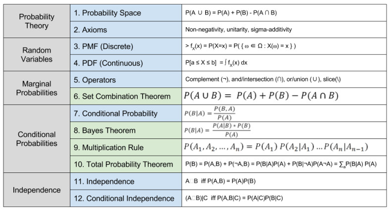
Probability theory, as formulated by Andrey Kolmogorov in 1925, has two ingredients:

1. A space which define the mathematical objects (“the nouns”)
2. Axioms which define the mathematical operations (“the verbs”)

A probability space is a 3-tuple (Ω,𝓕,P):

1. Sample Space (Ω): A set of possible outcomes, from one or more events. Outcomes in Ω must be mutually exclusive and collectively exhaustive.
2. σ-Algebra (𝓕). A collection of event groupings, or subsets. If Ω is countable, this can simply be the power set, otherwise a Borel algebra is often used.
3. Probability Measure Function (P). A real-valued function P: Ω → ℝ which maps from events to real numbers.

The Kolmogorov axioms provide “rules of behavior” for the residents of probability space:

1. Non-negativity: probabilities can never be negative, P(x) >= 0.
2. Unitarity: the sum of all probabilities is 1.0 (“something has to happen”)
3. Sigma Additivity: the probability of composite events equals the sum of their individual probabilities.

Random Variables

A random variable is a real-valued function X: Ω → ℝ. A random variable is a function, but not a probability function. Rather, instantiating random variables X = x defines a subset of events ⍵ ∈ Ω such that X(⍵) = x. Thus x picks out the preimage of Ω. Variable instantiation thus provides a language to select groups of events from Ω.

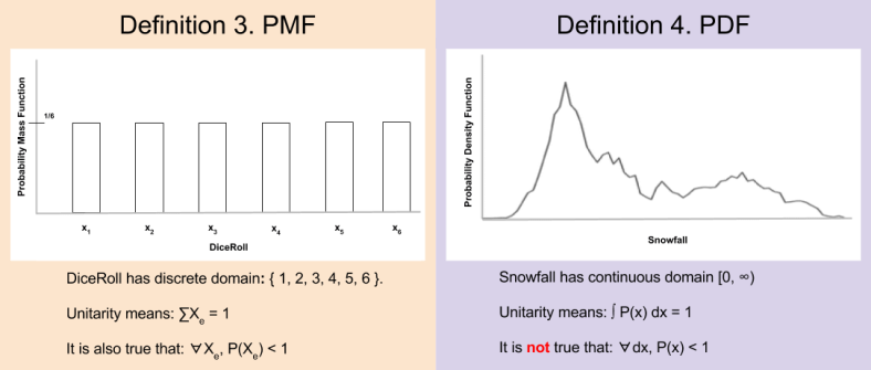
Random variables with discrete outcomes (countably finite Ω) are known as discrete random variable. We can define probability mass functions (PMFs) such that

In contrast, continuous random variables have continuous outcomes (uncountable Ω). For this class of variable, the probability of any particular event is undefined. Instead, we must define probabilities against a particular interval. The probability of 5.0000000… inches of snow is 0%; it is more meaningful to discuss the probability of 5 ± 0.5 inches of snowfall. Thus, we define probability density functions (PDFs) such that:

We can summarize discrete PMFs and continuous PDFs in the following graphic:

Marginal Probabilities

Consider two random variables, A and B ∈ Ω. Several operators may act on these variables, which parallel similar devices in Boolean algebra and set theory.

Suppose we want to know the probability of either A or B occurring. For this, we rely on the Set Combination Theorem:

Union involves subtracting the intersection; else the purple region is counted twice. In our post on set theory, we saw this same idea expressed as the inclusion-exclusion principle (Definition 13).

Summary

This first post in a two part explored the first six concepts or probability theory. Next time, we will learn about concepts 7-12.

These definitions and theorems are the cornerstone upon which much reasoning are built. It pays to learn them well.

Related Work

• https://ocw.mit.edu/courses/mathematics/18-05-introduction-to-probability-and-statistics-spring-2014/readings/MIT18_05S14_Reading3.pdf
• http://math.stackexchange.com/questions/690531/intuition-for-random-variable-being-sigma-algebra-measurable