Part Of: Optimization sequence
Content Summary: 800 words, 8 min read.

Today, I introduce the concept of duality. Buckle your seat belts! 🙂

Max Flow algorithm

The problem of flow was originally studied in the context of the USSR railway system in the 1930s. The Russian mathematician A.N. Tolstoy published his Methods of finding the minimal total kilometrage in cargo-transportation planning in space, where he formalized the problem as follows.

We interpret transportation graphically. Vertices are interpreted as cities, and edges are railroads connecting two cities. The capacity of each edge was the amount of goods that particular railroad could transport in a given day. The bottleneck is solely the capacities, and not production and consumption. We assume no available storage at the intermediate cities.

The flow allocation problem defines source and termination vertices, s and t. We desire to maximize volume of goods transported s → t. To do this, we label each edge with the amount of goods we intend to ship on that railroad. This quantity, which we will call flow, must respect the following properties:

• Flow cannot exceed the capacity of the railroad.
• Flow is conserved: stuff leaving a city must equal the amount of stuff arriving.

Here are two possible solutions to flow allocation:

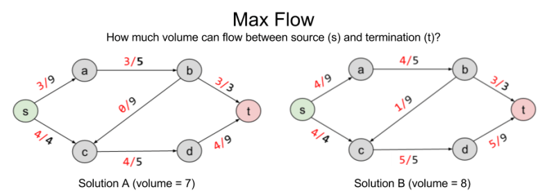
Solution B improves on A by pushing volume onto the b → c railway. But are there better solutions?

To answer rigorously, we formalize max flow as a linear optimization problem:

The solution to LP tells us that no, eight is the maximum possible flow.

Min Cut algorithm

Consider another, seemingly unrelated, problem we might wish to solve: separability. Let X ⊂ E represent the number of edges you need to remove to eliminate a connection s → t. Here are two such solutions:

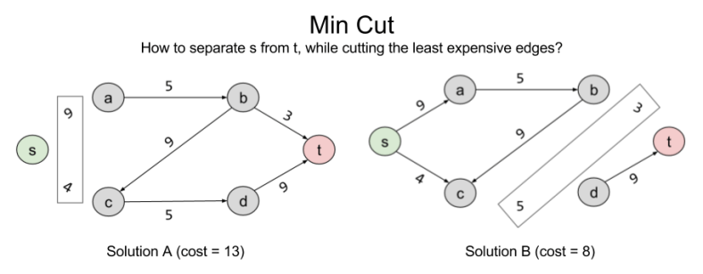
Can we do better than B? The answer is no: { (b,t), (c,d) } is the minimum cut possible in the current graph. In linear programming terms, it is the Best Feasible Solution (BFS)

Note that the BFS of minimum cut and the BFS of max flow arrive at the same value. 8 = 8. This is not a coincidence. In fact, these problems are intimately related to one another. What the min cut algorithm is searching for is the bottleneck: the smallest section of the “pipe” from s → t. For complex graphs like this, it is not trivial to derive this answer visually; but the separability algorithm does the work for us.

The deep symmetry between max flow and min cut demonstrates an important mathematical fact. All algorithms come in pairs. For this example, we will call max flow and min cut the primal and dual problems, respectively. We will explore the ramifications for this another time. For now, let’s approach duality from an algebraic perspective.

Finding LP Upper Bound

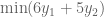
Consider a linear program with the following objective function:

And these constraints

This program wants to find the largest solution possible given constraints. Can we provide an upper bound on the solution?

Yes. We can immediately say that the solution is no greater than 6. Why? The objective function, is always smaller than , because we know all variables are positive. So we have an upper bound OPT ≤ 6. We can sharpen this upper bound, by comparing the objective function to other linear combinations of the constraints.  

Different weights to our linear combinations produce different upper bounds:

• (1,0) → 6
• (0,1) → 5
• (⅓, ⅓ ) → 3.67

Let us call these two weights . What values of these variables give us the smallest upper bound? Importantly, this is itself an objective function: .

But and are constrained: they must produce an equation that exceeds . Thus,

and 

This gives us our two constraints. Thus, by looking for the lowest upper bound on our primal LP, we have derived our dual LP:

Note the extraordinary symmetry between primal and dual LPs. The purple & orange values are mirror images of one another. Further, the constraint coefficient matrix has transposed (the 3 has swapped along the diagonal). This symmetry is reflected in the above linear algebra formulae. 

A Theory of Duality

Recall that linear programs have three possible outcomes: infeasible (no solution exists), unbounded (solution exists at +/-∞) or feasible/optimal. Since constraints are nothing more than geometric half-spaces, these possible outcomes reflect three kinds of polyhedra:

The outcome of primal and dual programs are predictably correlated. Of the nine potential pairings, only four can actually occur:

1. Both P and D are infeasible
2. P is unbounded and D is infeasible
3. D is unbounded and P is infeasible
4. Both are feasible, and there exist optimal solutions

Finally, in the above examples, we saw that the optimal dual value . But this is not always the case. In fact, the optimal dual value can be smaller .

We can distinguish between two kinds of duality:

• Strong duality, where
• Weak duality, where

Takeaways

Today, we have illustrated a deep mathematical fact: all problems come in pairs. Next time, we will explore the profound ramifications of this duality principle.

Related Resources: CMU Lecture 5: LP Duality