Part Of: Algebra sequence
Followup To: An Introduction to Geometric Group Theory
Content Summary: 1800 words, 18 min read
On Permutations
In the last few posts, we have discussed algebraic structures whose sets contain objects (e.g., numbers). Now, let’s consider structures over a set of functions, whose binary operation is function composition.
Definition 1. Consider two functions  and
and  . We will denote function composition of
  as
as  . We will use this notation instead of the more common
  . Both represent the idea “apply , then “.
Consider  .
.
Is this a group? Let’s check closure:
Closure is violated.  isn’t even a magma! Adding
  to the underlying set exacerbates the problem: then both
  and
and  .
.
So it is hard to establish closure under function composition. Can it be done?
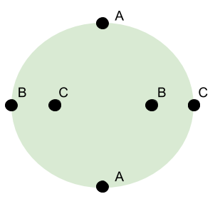
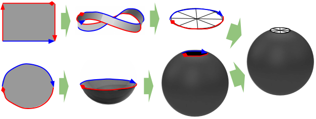
Yes. Composition exhibits closure on sets of permutation functions. Recall that a permutation is simply a bijection: it re-arrange a collection of things. For example, here are the six possible bijections over a set of three elements.

Definition 2. The symmetric group  denotes composition over a set of all bijections (permutations) over some set of
  objects. The symmetric group is then of order
  .
.
The underlying set of  is the set of all permutations over a 3-element set. It is of order
  .
.
This graphical representation of permutations is rather unwieldy. Let’s switch to a different notation system!
Notation 3: Two Line Notation. We can use two lines to denote each permutation mapping  . The top row represents the original elements
  , the bottom represents where each element has been relocated
  .
.
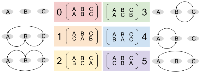
Two line notation is sometimes represented as an array, with the top row as matrix row, and bottom denoting matrix column. Then the identity matrix represents the identity permutation.
Definition 4. A cycle is a sequence of morphisms that forms a closed loop. An n-cycle is a cycle of length n. A 1-cycle does nothing. A 2-cycle is given the special name transposition.  has two permutations with 3-cycles: can you find them?
Theorem 5. Cycle Decomposition Theorem. Every permutation can be decomposed into disjoint cycles. Put differently, a node cannot participate in more than one cycle. If it did, its parent cycles would merge.
Notation 6: Cycle Notation. Since permutations always decompose into cycles, we can represent them as 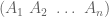 , pronounced “
 goes to
  goes to …”.
Cycle starting element does not matter:  .
.
The Cycle Algorithm
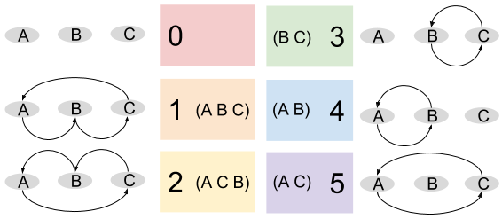
It is difficult to tell visually the outcome of permutation composition. Let’s design an algorithm to do it for us!
Algorithm 7: Cycle Algorithm. To compose two permutation functions  and
and  , take each element
  and follow its arrows until you find the set of disjoint cycles. More formally, compose these functions times until you get
  .
.
Here’s a simple example from  .
.

Make sense? Good! Let’s try a more complicated example from  .
.
A couple observations are in order.
- 1-cycles (e.g.,
 ) can be omitted: their inclusion does not affect algorithm results.
- Disjoint cycles commute:
 . Contrast this with composition, which does not commute
  .
.
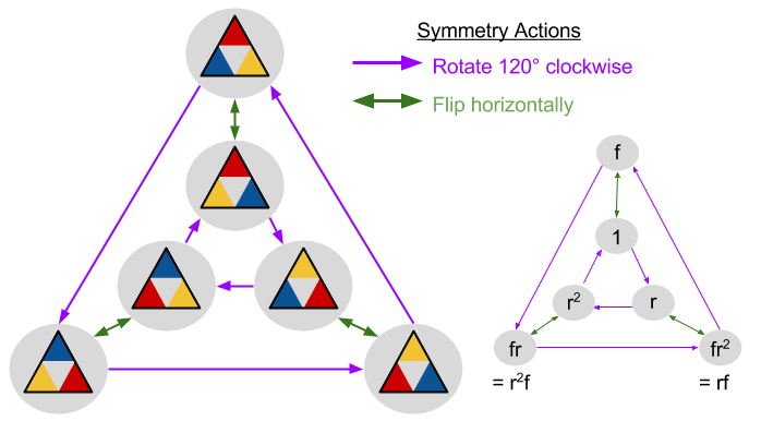
Now, let’s return to for a moment, with its set of six permutation functions. Is this group closed? We can just check every possible composition:

From the Cayley table on the right, we see immediately that is closed (no new colors) and non-Abelian (not diagonal-symmetric).
But there is something much more interesting in this table. You have seen it before. Remember the dihedral group  ? It is isomorphic to !
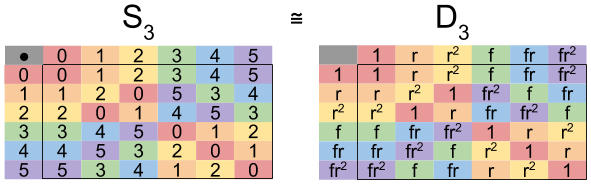
If you go back to the original permutation pictures, this begins to make sense. Permutations  and
and  resemble rotations/cycles;
  ,
,  , and
, and  perform reflections/flips.
Generators & Presentations
In Theorem 7, we learned that permutations decompose into cycles. Let’s dig deeper into this idea.
Theorem 8. Every n-cycle can be decomposed into some combination of 2-cycles. In other words, cycles are built from transpositions.
The group  has three transpositions
  ,
,  , and
, and  .
.
Transpositions are important because they are generators: every permutation can be generated by them. For example,  . In fact, we can lay claim to an even stronger fact:
Theorem 9. Every permutation can be generated by adjacent transpositions. Every permutation  .
.
By the isomorphism  , we can generate our “dihedral-looking” Cayley graph by selecting generators
  and
and  .
.
But we can use Theorem 9 to produce another, equally valid Cayley diagram. There are two adjacent transpositions in : and . All other permutations can be written in terms of these two generators:
This allows us to generate a transposition-based Cayley diagram. Here are the dihedral and transposition Cayley diagrams, side by side:

We can confirm the validity of the transposition diagram by returning to our multiplication table:  means a green arrow
  .
.
Note that the transposition diagram is not equivalent cyclic group  , because arrows in the latter are monochrome and unidirectional.
We’re not quite done! We can also rename our set elements to employ generator-dependent names, by “moving clockwise”:

We could just as easily have “moved counterclockwise”, with names like  ,
,  . And we can confirm by inspection that, in fact,
  etc.
etc.
Using the original clockwise notation, one presentation of becomes:

Towards Alternating Groups
Any given permutation can be written as a product of permutation. Consider, for example, the above equalities
 . These have 2, 4, and 8 permutations, respectively.
  . These have 3, 5, and 9 permutations, respectively.
Did you notice any patterns in the above lists? All expressions for require an even number of transpositions, and all expressions of require an odd number. In other words, the parity (evenness or oddness) of a given permutation doesn’t seem to be changing. In fact, this observation generalizes:
Theorem 10. For any given permutation, the parity of its transpositions is unique.
Thus, we can classify permutations by their parity. Let’s do this for :
 are even permutations.
 of odd permutations.
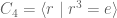
Theorem 11. Exactly half of are even permutations, and they form a group called the alternating group  . Just as
  , has
, has  elements.
Why don’t odd permutations form a group? For one thing, it doesn’t contain the identity permutation, which is always even.
Let’s examine 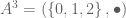 in more detail. Does it remind you of anything?
It is isomorphic to the cyclic group  ..!
..!

We have so far identified the following isomorphisms: and  . Is it also true that e.g.,
  and
and  ?
?
No! Recall that the  and
and  . Only
  , these sets are not even potentially isomorphic. For example:
 .
. .
.
For these larger values of , the symmetric group is much larger than dihedral and cyclic groups.
Applications
Why do symmetric & alternating groups matter? Let me give two answers.
Perhaps you have seen the quadratic equation, the generic solution to quadratic polynomials  .
.
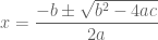
Analogous formulae exist for cubic (degree-3) and quartic (degree-4) polynomials. 18th century mathematics was consumed by the theory of equations: mathematicians attempting to solve quintic polynomials (degree-5). Ultimately, this quest proved to be misguided: there is no general solution to quintic polynomials.
Why should degree-5 polynomials admit no solution? As we will see when we get to Galois Theory, it has to do with the properties of symmetric group  .
.
A second reason to pay attention to symmetric groups comes from the classification theorem of finite groups. Mathematicians have spent decades exploring the entire universe of finite groups, finding arcane creatures such as the monster group, which may or may not explain features of quantum gravity.
One way to think about group space is by the following periodic table:

Image courtesy of Samuel Prime.
Crucially, in this diverse landscape, the symmetric group plays a unique role:
Theorem 12: Cayley’s Theorem. Every finite group is a subgroup of the subgroup , for some sufficiently large .
For historical reasons, subgroups of the symmetric group are usually called permutation groups.
Until next time.
Wrapping Up
Takeaways:
- The symmetric group is set of all bijections (permutations) over some set of objects, closed under function composition.
- Permutations can be decomposed into disjoint cycles: cycle notation uses this fact to provide an algorithm to solve for arbitrary compositions.
- All permutations (and hence, the symmetric group) can be generated by adjacent transpositions. This allows us to construct a presentation of the symmetric group.
- Permutations have unique parity: thus we can classify permutations as even or odd. The group of even presentations is called the alternating group .
- It can be shown that and
 . However, for larger , the symmetric and alternating group are much larger than cyclic and dihedral groups.
The best way to learn math is through practice! If you want to internalize this material, I encourage you to work out for yourself the Cayley table & Cayley diagram for . 🙂
Related Resources
For a more traditional approach to the subject, these Harvard lectures are a good resource.


![[ -30, 30, -30, 30]](https://s0.wp.com/latex.php?latex=%5B+-30%2C+30%2C+-30%2C+30%5D&bg=ffffff&fg=555555&s=0&c=20201002)
![[0, 0, 0, 0]](https://s0.wp.com/latex.php?latex=%5B0%2C+0%2C+0%2C+0%5D&bg=ffffff&fg=555555&s=0&c=20201002)
![[ 1, -1, 1, -1, 1, -1 ]](https://s0.wp.com/latex.php?latex=%5B+1%2C+-1%2C+1%2C+-1%2C+1%2C+-1+%5D&bg=ffffff&fg=555555&s=0&c=20201002)
![[ 3, -3 ]](https://s0.wp.com/latex.php?latex=%5B+3%2C+-3+%5D&bg=ffffff&fg=555555&s=0&c=20201002)


 with
with  possible outcomes, and another event
  with
with  is
is  .
.  possible outcomes.
  possible outcomes.
  possible outcomes.
 possible trifecta bets.

 . How can we get rid of the other terms? By division, of course!


 possible trifecta bets. But how many
  and
and  are equivalent for a boxed trifecta bet. We can identify four groups, with six equivalent permutations each:
 !
!
 cookies
  to give to
  kids. How many possible ways are there to do so?
 ,
,  ,
,  , and
, and  . But there is an important difference: horse-less medals are impossible, but cookie-less children are not! So we need to account for situations like
  , with one child getting all of the cookies.
 .
. bars. Thus:


 .
. and
and  . A single horse cannot win multiple medals. Multiply-realized possibilities are not allowed.


 .
. .
. .
.  ). Are finite groups possible?
 . Is it a group? No, it isn’t even a magma:
  ! Is there a different operation that would produce closure?
  , on
, on  . For example,
  .
.
 .
. is an
is an  . Its solutions, or roots, is the set
  . This set is called the fourth roots of unity.
 ? In the following table, recall that
  , thus
  .
.
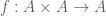 . Let’s compare the function maps of our two groups:
 . Let
. Let .
.
 . Inspection reveals that this, too, is isomorphic to
  !
! , there exists some generator
  , where r is any generator.
 .
.
 . But you can also recreate them by
  .
.  , or multiplying by
  . Only
  fails to be a generator.
  rotation, and counterclockwise
  .
. .
. .
.  ? All non-identity elements:
  .
.  .
. configurations. It would take a long time just writing down such a group. But it has only six generators (one for a
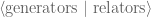
 .
. .
. suffix is often left implicit from presentations (e.g.,
  ) for the sake of concision.
 . Let us consider the “triangle group”
  rotation
  and a horizontal flip
  . Similarly, two flips returns to the identity
  . Is there some combination of rotations
 .
.
 .
.

 is not abelian: its multiplication table is not symmetric about the diagonal.
 table with a
  table. We will explore this intuition further, when we discuss quotients.
 and
and  When do we call these lines parallel? When their slopes are equal
  . We can gain insight into the situation by mapping
  and
and  form the horizontal and vertical axes respectively.
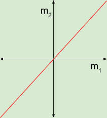
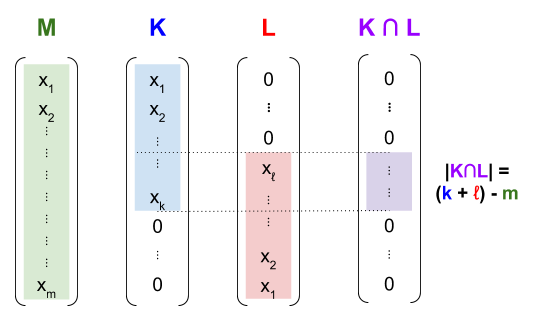
 and
and  being placed in an
  . We denote their intersection as
  . Let us compare the dimensions of these three manifolds to the dimension of their overlap.
  as
as  respectively. Now our examples can be expressed as 4-tuples
  :
:


 ?
?  , that the two planes intersect at a point, you have noticed the pattern!
  . The overflow is defined as
 , the submanifolds do not intersect:
 , the intersection is non-empty
  , and
, and 
 vs.
vs.  vs.
vs.  vs.
vs.  vs.
vs.  vs.
vs.  :
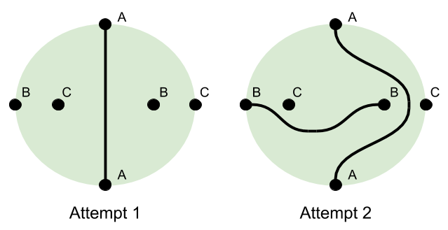
: , then generically, a crossing is possible (at all times,
  , then generically, a crossing is not possible (at some time,
  is the following movement possible?
 . But Theorem 4 says that, if the ambient dimension is four, then the overflow is
 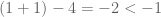 , so crossing is possible.
 and
and  represent the beginning and end positions as it travels throughout time
 ![t \in [0,1]](https://s0.wp.com/latex.php?latex=t+%5Cin+%5B0%2C1%5D&bg=ffffff&fg=555555&s=0&c=20201002) . If
. If  never has self-intersection at any time
  , we say
 : this is why it is called
  : we can unwind the trefoil knot in
  : simply lift the top-left string up.
  to
to  : you only need
 , knots self-intersect. In
 ; after all
  .
. :
:
 ). If we isotope along its surface using
  , is
, is  ? How about
  ?
? 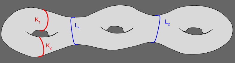
 . You just pull the circle left, along that surface of the torus.
 . You might suspect you can just pull the blue circle over the middle hole. But that would require leaving the surface
  (but
(but  ).
). represents the set of fruits which I prefer.
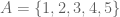 can represent, among other things, the fingers on my left hand.
 .
. .
. and
and  expresses the very same set.
  . We will prefer to express sets with the latter, more compact, notation.
 is a perfectly valid two-element set, quite distinct from the three-element set
  .
. ) if A and B contain exactly the same elements.
 and
and  . Then,
  . Then,
  .
. . Otherwise, we write
  .
. . Then
  means “yellow is an element of the set of primary colors”.
 means “-1 is not an element of the natural numbers”.
 . The element
  is.
is. , its
, its  , is the number of elements in that set.
 .
. . Then
  . Note that cardinality only looks at “the outer layer”.
  is the set containing no elements.
  .
. .
. .
.  , where the | symbol is pronounced “such that”.
 . In words “let A be the set of integers X such that x is greater than zero and less than six.”
 .
. and let
  . Here
  bits of computer memory, each bit of which is uniquely identified with a 6-bit address. Suppose further that our memory has been allocated to data structures of varying size. To promote addressing efficiency, a computer can adopt the following strategy: assign shorter addresses to larger variables.
 , if every element of
  and
and  . Then
  . Then
  (C does not contain 9).
 ? Yes. For all
  is true.
 , if
, if  is the set of all subsets of
  . Then
  .
.
 , then
  .
. ) versus subset-of (
  ) relations. Consider again
  . But
. But  . The
. The  . But
. But  . The
. The  -algebras draw from the power set of natural numbers
  .
. is the set of all
  such that
  and
and  . Note that, unlike the elements in a set, the elements of an ordered pair cannot be reordered.
 and
and  . Then
  .
.
 . Thus,
  . This is because elements within ordered pairs cannot be rearranged.
 . In combinatorics, this observation generalizes to the multiplication principle.
 is a well-known example of a Cartesian product.
 , their Cartesian product is the set of all n-tuples.
 ,
,  and
and  . Now
. Now  .
. , is the set of elements common to both sets.
 and
and  . Then
  .
. . Then
  .
. .
. .
. .
.

 . This
  is the set of elements in
  and
and  . Then
  and
and  .
. . Then
  and
and  .
. is the set of elements in
  .
.
 and let its universe be the set of complex numbers
  . It is true that
  .
. is the set of all elements of
  and
and  .
.


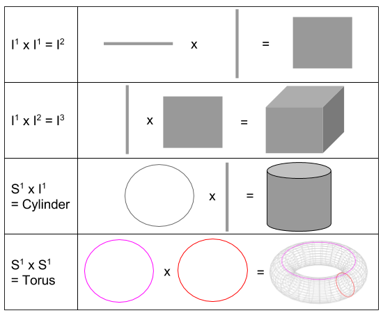
 is a line segment
 is a
is a  is a
is a  is a
is a  makes the volume-surface relationship explicit. For example, we say that
  .
.


 :
:


