Part Of: Machine Learning sequence
Followup To: Regression vs Classification
Content Summary: 800 words, 8 min read

A Taxonomy of Models

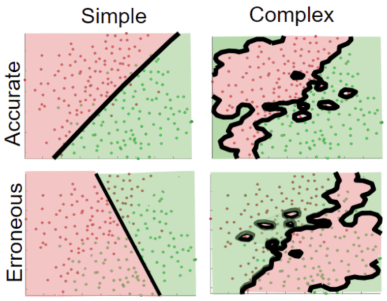
Last time, we discussed how to create prediction machines. For example, given an animal’s height and weight, we might build a prediction machine to guess what kind of animal it is. While this sounds complicated, in this case prediction machines are simple region-color maps, like these:

These two classification models are both fairly accurate, but differ in their complexity. 

But it’s important to acknowledge the possibility of erroneous-simple and erroneous-complex models. I like to think of models in terms of an accuracy-complexity quadrant.

This quadrant is not limited to classification. Regression models can also vary in their accuracy, and their complexity.

A couple brief caveats before we proceed.

• This quadrant concept is best understood as a two-dimensional continuum, rather than a four-category space. More on this later.
• Here “accuracy” tries to capture lay intuitions about prediction quality & performance. I’m not using it in the metric sense of “alternative to F1 score”.

Formalizing Complexity

Neural networks are often used as classification models against large numbers of images. The complexity of the models tends to correlate with the number of layers. For some models then, complexity is captured in the number of parameters.

While not used much in the industry, polynomial models are pedagogically useful examples of regression models. Here, the degree of the polynomial expresses the complexity of the model: a degree-eight polynomial has more “bumps” than a degree-two polynomial.

Consider, however, the difference between the following regression models

Model A uses five parameters; Model B uses three. But their predictions are, for all practical purposes, identical. Thus, the size of each parameter is also relevant to the question of complexity.

The above approaches rely on the model’s parameters (its “visceral organs”) to define complexity. But it is also possible to rely on the model’s outputs (its “behaviors”) to achieve the same task. Consider again the classification decision boundaries above. We can simply measure the spatial frequency (the “squiggliness” of the boundary) as another proxy towards complexity.

Here, then, are three possible criteria for complexity:

1. Number of parameters
2. Size of parameters
3. Spatial frequency of decision manifold

Thus, operationalizing the definition of “complexity” is surprisingly challenging. But there is another way to detect whether a model is too complex…

Simplicity as Generalizability

Recall our distinction between training and prediction:

We compute model performance on historical data. We can contrast this with model performance again future data. 

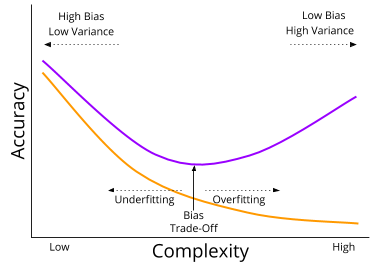
Take a moment to digest this image. What is it telling you?

Model complexity is not merely aesthetically ugly. Rather, complexity is the enemy of generalization. Want to future-proof your model? Simplicity might help!

Underfitting vs Overfitting

There is another way of interpreting this tradeoff, that emphasizes the continuity of model complexity. Starting from a very simple model, increases in model complexity will improve both historical and future error. The best response to underfitting is increasing the expressivity of your model.

But at a certain point, your model will become too complex, and begin to overfit the data. At that point, your historical error will continue to decrease, but your future error will increase.

Data Partitioning: creating a Holdout Set

So you now appreciate the importance of striking a balance between accuracy and simplicity. That’s all very nice conceptually, but how might you go about building a well-balanced prediction machine?

The bias trade-off is only apparent when the machine is given new data!  “If only I had practiced against unseen test data earlier”, the statistician might say, “then I could have discovered how complex to make my model before it was too late”.

Read the above regret again. It is the germinating seed of a truly enormous idea.

Many decades ago, some creative mind took the above regret and sought to reform it: “What stops me from treating some of my old, pre-processed data as if it were new? Can I not hide data from myself?”

This approach, known as data partitioning, is now ubiquitous in the machine learning community.  Historical-Known data is the training set, Historical-Novel data is the test set, aka the holdout set.

How much data should we put in the holdout set? While the correct answer ultimately derives from the particular application domain, a typical rule of thumb:

• On small data (~100 thousand records), data are typically split to 80% train, 20% test
• On large data (~10 billion records), data are typically split to 95% train, 5% test

Next time, we will explore cross-validation (CV). Cross-validation is sometimes used instead of, and other times in addition to, data partitioning.

See you then!