An Introduction to Language Models

Part Of: Language sequence
Content Summary: 1500 words, 15 min read

Why Language Models?

In the English language, ‘e’ appears more frequently than ‘z’. Similarly, “the” occurs more frequently than “octopus”. By examining large volumes of text, we can learn the probability distributions of characters and words.

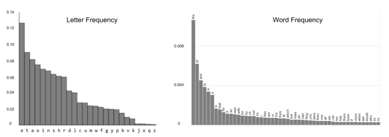
Language Models_ Letter and Word Frequency

Roughly speaking, statistical structure is distance from maximal entropy. The fact that the above distributions are non-uniform means that English is internally recoverable: if noise corrupts part of a message, the surrounding can be used to recover the original signal. Statistical structure is also used to reverse engineer secret codes such as the Roman cipher.

We can illustrate the predictability of English by generating text based on the above probability distributions. As you factor in more of the surrounding context, the utterances begin to sound less alien, and more like natural language.

Language Model_ Structure of English

A language model exploits the statistical structure of a language to express the following:

Assign a probability to a sentence $P(w_1, w_2, w_3, \ldots w_N)$
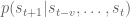
Assign probability of an upcoming word $P(w_4 \mid w_1, w_2, w_3)$

Language models are particularly useful in language perception, because they can help interpret ambiguous utterances. Three such applications might be,

Machine Translation: $P(\text{high winds tonight}) > P(\text{large winds tonight})$
Spelling correction: $P(\text{fifteen minutes from}) > P(\text{fifteen minuets from})$
Speech Recognition: $P(\text{I saw a van}) > P(\text{eyes awe of an})$

Language models can also aid in language production. One example of this is autocomplete-based typing assistants, commonly displayed within text messaging applications.

Towards N-Grams

A sentence is a sequence of words 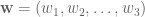$\textbf{w} = (w_1, w_2, \ldots, w_3)$ . To model the joint probability over this sequence, we use the chain rule:

$p(\text{this is the house})$

$= p(\text{this})p(\text{is}\mid\text{this})p(\text{the}\mid\text{this is})p(\text{house}\mid\text{this is the})$

As the number of words grows, the size of our conditional probability tables (CPTs) quickly becomes intractable. What is to be done? Well, recall the Markov assumption we introduced in Markov chains.

markov_assumption

The Markov assumption constrains the size of our CPTs. However, sometimes we want to condition on more (or less!) than just one previous word. Let $v$ denote how many variables we admit in our context. A variable order Markov model (VOM) allows $v$ elements in its context: $p(s_{t+1} | s_{t-v}, \ldots, s_{t})$ . Then the size of our CPT is $n=v+1$ , because we must take our original variable into account. Thus an N-gram is defined as a $v$ -order Markov model. By far, the most common choices are trigrams, bigrams, and unigrams:

Language Models_ Ngram comparison (1)

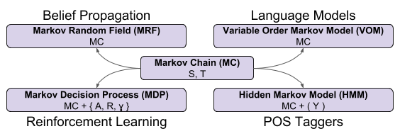
We have already discussed Markov Decision Processes, used in reinforcement learning applications. We haven’t yet discussed MRFs and HMMs. VOMs represent a fourth extension: the formalization of N-grams. Hopefully you are starting to appreciate the richness of this “formalism family”. 🙂

Language Model_ Markov Formalisms (1)

Estimation and Generation

How can we estimate these probabilities? By counting!

ngram_v2

Let’s consider a simple bigram language model. Imagine training on this corpus:

This is the cheese.

That lay in the house that Alice built.

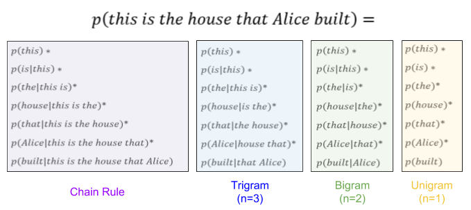
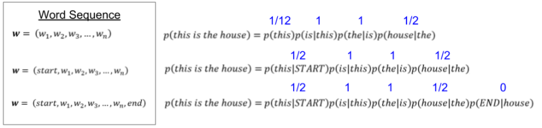
Suppose our trained LM encounters the new sentence “this is the house”. It estimates its probability as:

$p(\text{this is the house})$

$= p(\text{this})p(\text{is} \mid \text{this})p(\text{the} \mid \text{is})p(\text{house} \mid \text{the})$

$= \dfrac{1}{12} * 1 * 1 * \dfrac{1}{2} = \dfrac{1}{24}$

How many problems do you see with this model? Let me discuss two.

First, we have estimated that $p(\text{this}) = \dfrac{1}{24}$ . And it is true that “this” occurs only once in our toy corpus above. But out of two sentences, “this” leads half of them. We can express this fact by adding a special START token into our vocabulary.

Second, recall what happens when language models generate speech. Once they begin a sentence, they are unable to end it! Adding a new END token will allow our model the terminate a sentence, and begin a new one.

With these new tokens in hand, we update our products as follows:

Language Models_ Sentence Estimation (1)

A couple other “bug fixes” I’ll mention in passing:

Out-of-vocabulary words are given zero probability. It helps to add an unknown (UNK) pseudoword and assign it some probability mass.
LMs prefer very short sentences (sequential multiplication is monotonic decreasing). We can address this e.g., normalizing by sentence length.

Smoothing

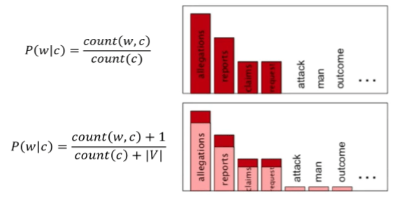
In the last sentence in the image above, we estimate 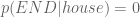$p(END|house) = 0$ , because we have no instances of this two-word sequence in our toy corpus. But this causes our language model to fail catastrophically: the sentence is deemed impossible (0% probability).

This problem of zero probability increases as we increase the complexity of our N-grams. Trigram models are more accurate than bigrams, but produce more $p=0$ events. You’ll notice echoes of the bias-variance (accuracy-generalization) tradeoff.

How can we remove zero counts? Why not add one to every word? Of course, we’d then need to increase the size of our denominator, to ensure the probabilities still sum to one. This is Laplace smoothing.

Language Model_ Laplace Smoothing

In a later post, we will explore how (in a Bayesian framework) such smoothing algorithms can be interpreted as a form of regularization (MAP vs MLE).

Due to its simplicity, Laplace smoothing is well-known But several algorithms achieve better performance. How do they approach smoothing?

Recall that a zero count event in an $N$ -gram is not likely to occur in $(N-1)$ -gram model. For example, it is very possible that the phrase “dancing were thought” hasn’t been seen before.

Language Model_ Backoff Smoothing

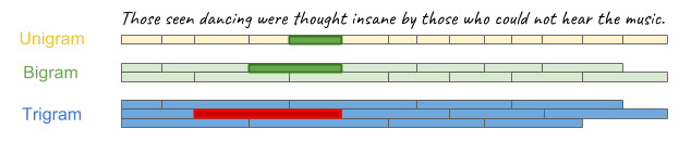
While a trigram model may balk at the above sentence, we can fall back on the bigram and/or unigram models. This technique underlies the Stupid Backoff algorithm.

As another variant on this theme, some smoothing algorithms train multiple $N$ -grams, and essentially use interpolation as an ensembling method. Such models include Good-Turing and Kneser-Ney algorithms.

Beam Search

We have so far seen examples of language perception, which assigns probabilities to text. Let us consider language perception, which generates text from the probabilistic model. Consider machine translation. For a French sentence $\textbf{x}$ , we want to produce the English sentence $\textbf{y}$ such that $y^* = \text{argmax } p(y\mid x)$ .

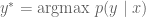
This seemingly innocent expression conceals a truly monstrous search space. Deterministic search has us examine every possible English sentence. For a vocabulary size $V$ , there are $V^2$ possible two-word sentences. For sentences of length $n$ , our time complexity of our brute force algorithm is $O(V^n)$ .

Since deterministic search is so costly, we might consider greedy search instead. Consider an example French sentence $\textbf{x}$ “Jane visite l’Afrique en Septembre”. Three candidate translations might be,

$y^A$ : Jane is visiting Africa in September
$y^B$ : Jane is going to Africa in September
$y^C$ : In September, Jane went to Africa

Of these, $p(y^A|x)$ is the best (most probable) translation. We would like greedy search to recover it.

Greedy search generates the English translation, one word at a time. If “Jane” is the most probable first word $\text{argmax } p(w_1 \mid x)$ , then the next word generated is $\text{argmax } p(w_2 \mid \text{Jane}, x)$ . However, it is not difficult to contemplate $p(\text{going}\mid\text{Jane is}) > p(\text{visiting}\mid\text{Jane is})$ , since the word “going” is used so much more frequently in everyday conversation. These problems of local optima happen surprisingly often.

The deterministic search space is too large, and greedy search is too confining. Let’s look for a common ground.

Beam search resembles greedy search in that it generates words sequentially. Whereas greedy search only drills one such path in the search tree, beam search drills a finite number of paths. Consider the following example with beamwidth $b=3$

beam_search

As you can see, beam search elects to explore $y^A$ as a “second rate” translation candidate despite $y^B$ initially receiving the most probability mass. Only later in the sentence does the language model discover the virtues of the $y^A$ translation. 🙂

Strengths and Weaknesses

Language models have three very significant weaknesses.

First, language models are blind to syntax. They don’t even have a concept of nouns vs. verbs! You have to look elsewhere to find representations of pretty much any latent structure discovered by linguistic and psycholinguistic research.

Second, language models are blind to semantics and pragmatics. This is particularly evident in the case of language production: try having your SMS autocomplete write out an entire sentence for you. In the real world, communication is more constrained: we choose the most likely word given the semantic content we wish to express right now.

Third, the Markov assumption is problematic due to long-distance dependencies. Compare the phrase “dog runs” vs “dogs run”. Clearly, the verb suffix depends on the noun suffix (and vice versa). Trigram models are able to capture this dependency. However, if you center-embed prepositional phrases, e.g., “dog/s that live on my street and bark incessantly at night run/s”, N-grams fail to capture this dependency.

Despite these limitations, language models “just work” in a surprising diversity of applications. These models are particularly relevant today because it turns out that Deep Learning sequence models like LSTMs share much in common with VOMs. But that is a story we shall have to take up next time.

Until then.

Fewer Lacunae

Distilled, Integrative Research

An Introduction to Language Models

Leave a Reply Cancel reply

Share this:

Like this:

Related

Leave a Reply Cancel reply