[Video] An introduction to reinforcement learning

Part Of: Reinforcement Learning sequence

Sorry it’s been so long since my last post!  I’ve been teaching a Deep Learning class, based on Andrew Ng’s Coursera specialization.  Don’t worry, my other lectures will ultimately be cleaned & shared here too 🙂

This talk covers the mathematical intuitions of RL, which draws from content relating to Markov Chains and Markov Decision Processes. It also contains some novel material, including my thoughts on how RL compares with other machine learning techniques.


Advertisement

Markov Decision Processes

Part Of: Reinforcement Learning sequence
Followup To: An Introduction To Markov Chains
Content Summary: 900 words, 9 min read

Motivations

Today, we turn our gaze to Markov Decision Processes (MDPs), a decision-making environment which supports our propensity to learn from good and bad outcomes. We represent outcome desirability with a single number, R. This value is used to refine action selection: given a particular situation, what action will maximize expected reward?

In biology, we can describe the primary work performed by an organism is to maintain homeostasis: maintaining metabolic energy reserves, body temperature, etc in a widely varying world. 

Cybernetics provide a clear way of conceptualizing biological reward. In Neuroendocrine Integration, we discussed how brains must respond both to internal and external changes. This dichotomy expresses itself as two perception-action loops: a visceral body-oriented loop, and a cognitive world-centered one.

Rewards are computed by the visceral loop. To a first approximation, reward encode progress towards homeostasis. Food is perceived as more rewarding when the body is hungry, this is known as alliesthesia. Reward information is delivered to the cognitive loop, which helps refine its decision making.

Reinforcement Learning- Reward As Visceral Efferent

Extending Markov Chains

Recall that a Markov Chain contains a set of states S, and a transition model P. A Markov Decision Process (MDP) extends this device, by adding three new elements.

Specifically, an MDP is a 5-tuple (S, P, A, R, ɣ):

  • A set of states s ∈ S
  • A transition model Pa(s’ | s).
  • A set of actions a ∈ A
  • A reward function R(s, s’)
  • A discount factor ɣ

To illustrate, consider GridWorld. In this example, every location in this two-dimensional grid is a state, for example (1,0). State (3,0) is a desirable location: R(s(3,0)) = +1.0, but state (3,1) is undesirable, R(s(3,1)) = -1.0. All other states are neutral.

Gridworld supports four actions, or movements: up, down, left, and right.  However, locomotion is imperfect: if Up is selected, the agent will only move up with 80% probability: 20% of the time it will go left or right instead. Finally, attempting to move into a forbidden square will simply return the agent to its original location (“hitting the wall”).

Reinforcement Learning- Example MDP Gridworld

The core problem of MDPs is to find a policy (π), a function that specifies the agent’s response to all possible states. In general, policies should strive to maximize reward, e.g., something like this:

Reinforcement Learning- Example MDP Policy

Why is the policy at (2,2) Left instead of Up? Because (2,1) is dangerous: despite selecting Up, there is a 10% chance that the agent will accidentally move Right, and be punished.

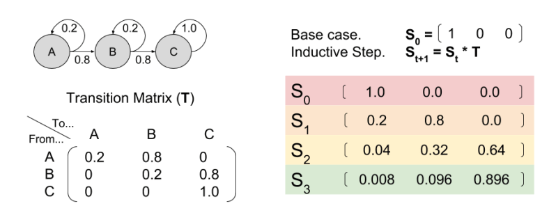
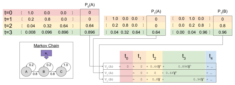
Let’s now consider an environment with only three states A, B, and C.  First, notice how different policies change the resultant Markov Chain:

reinforcement-learning-policy-vs-markov-chain-1

This observation is important. Policy determines the transition model.

Towards Policy Valuation V(s)

An agent seeks to maximize reward. But what does that mean, exactly?

Imagine an agent selects 𝝅1. Given the resultant Markov Chain, we already know how to use matrix multiplication to predict future locations St. The predicted reward Pt is simply the dot product of expected location and the reward function. 

P_t = S_t \cdot R

markov-chains-linear-algebra-expected-value

We might be tempted to define the value function V(S) as the sum of all predicted future rewards:

V_O(S) = P_0 + P_1 + P_2 + P_3 + \dots = \sum{P_k}

However, this approach is flawed.  Animals value temporal proximity: all else equal, we prefer to obtain rewards quickly. This is temporal discounting: as rewards are further removed from the present, their value is discounted. 

In reinforcement learning, we implement temporal discounting with the gamma parameter: rewards that are k timesteps away are multiplied by the exponential discount factor \gamma^k. The value function becomes:

V_O(S) = P_0 + \gamma P_1 + \gamma^2 P_2 + \gamma^3 P_3 + \dots = \sum{\gamma^k P_k}

Without temporal discounting, V(s) can approach infinity. But exponential discounting ensures V(s) equals a finite valueFinite valuations promote easier computation and comparison of state evaluations. For more on temporal discounting, and an alternative to the RL approach, see An Introduction to Hyperbolic Discounting.

Intertemporal Consistency

In our example, at time zero our agent starts in state A. We have already used linear algebra to compute our Pk predictions. To calculate value, we simply compute $latex \sum{\gamma^k P_k}$

V_0(A) = 0 + 0 + 0.64 \gamma^2 + 0.896 \gamma^3

Agents compute V(s) at every time step. At t=1, two valuations are relevant:

V_1(A) = 0 + 0 + 0.64 \gamma^2 + \dots

V_1(B) = 0 + 0.8 \gamma + 0.96 \gamma^2 + \dots

mdp-value-function-timeslice

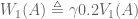
What is the relationship between the value functions at t=0 and t=1? To answer this, we need to multiply each term by \gamma P(X|A), where X is the state being considered at the next time step.

W_1(A) \triangleq \gamma 0.2 V_1(A)

W_1(A) = 0 + 0 + (0.2)(0.64)\gamma^3 + \dots

Similarly,

W_1(B) \triangleq \gamma P(B|A)V_1(B) = \gamma 0.8 V_1(B)

W_1(B) 0 + (0.8)(0.8) \gamma^2 + (0.8)(0.96) \gamma^3 + \dots

Critically, consider the sum X = r_0(s) + W_1(A) + W_1(B):

X = 0 + 0 + 0.64 \gamma^2 + 0.896 \gamma^3 + \dots

MDP- Intertemporal Consistency

Does X_0 look familiar? That’s because it equals V_0(A)! In this way, we have a way of equating a valuation at t=0 and t=1. This property is known as intertemporal consistency.

Bellman Equation

We have seen that V_0(A) = X_0. Let’s flesh out this equation, and generalize to time t.

V_t(s) = r_t(A) + \gamma \sum{P(s'|s)V_{t+1}(s')}

This is the Bellman Equation, and it is a central fixture in control systems. At its heart, we define value in terms of both immediate reward and future predicted value. We thereby break up a complex problem into small subproblems, a key optimization technique that can be approached with dynamic programming.

Next time, we will explore how reinforcement learning uses the Bellman Equation to learn strategies with which to engage its environment (the optimal policy 𝝅). See you then!

Iterated Schizophrenic’s Dilemma

Part Of: Breakdown of Will sequence
Followup To: Rule Feedback Loops
Content Summary: 1300 words, 13 min read

Context

Here’s where we landed last time:

  • Preference bundling is mentally implemented via a database of personal rules (“I will do X in situations that involve Y).
  • Personal rules constitute a feedback loop, whereby rule-compliance strengthen (and rule-circumvention weakens) the circuit.

Today’s post will draw from the following:

  1. An Introduction To Hyperbolic Discounting discusses warfare between successive selves (e.g., OdysseusNOW restricts the freedoms of OdysseusFUTURE in order to survive the sirens).
  2. An Introduction To Prisoner’s Dilemma discusses how maths can be used to describe the outcome of games between competitors.

Time to connect these threads! 🙂 Let’s ground our warfare narrative in the formal systems of game theory.

Schizophrenic’s Dilemma

First, we interpret { larger-later (LL) vs. smaller-sooner (SS) } rewards in terms of { cooperation vs. defection } decisions.

Second, we name our actors:

  • P represents your present-self
  • F represents your future-self
  • FF represents your far-future-self, etc.

Does this game suffer from the same issue as classical PD? Only one way to find out!

ISD- Simple Example (1)

Here’s how I would explain what’s going on:

  • Bold arrows represent decisions, irreversible choices in the real world. Decisions lock in final scores (yellow boxes).
  • Skinny arrows represent intentions, the construction of rules for future decisions.
  • The psychological reward you get from setting intentions is just as real as that produced by decisions.
  • Reward is accretive: your brain seeks to maximize the sum total reward it receives over time.

Take some time to really ingest this diagram.

Iterated Schizophrenic’s Dilemma (ISD)

Okay, so we now understand how to model intertemporal warfare as a kind of “Schizophrenic’s Dilemma“. But we “have to live with ourselves” — the analogy ought to be extended across more than one decision. Here’s how:

ISD - From Flat Behavior To IPD

Time flows from left to right. In the first row, we see that an organism’s choices are essentially linear. For each choice, the reasoner selects either an LL (larger-longer) or an SS (smaller-sooner) reward. How can this be made into a two-dimensional game? We can achieve this graphically by “stretching each choice point up and to the left”. This move ultimately implements the following:

  • Temporal Continuity: “the future-self of one time step must be equivalent to the present-self of the next time step”.

It is by virtue of this rule that we are able to conceptualize the present-self competing against the future-self (second row). The third row simply compresses the second into one state-space.

Let us call this version of the Iterated Prisoner’s Dilemma, the Iterated Schizophrenic’s Dilemma. For the remainder of this article, I will use IPD and ISD to distinguish between the two.

The Lens Of State-Space

We have previously considered decision-space, and outcome-space. Now we shall add a third space, what I shall simply call state-space (very similar to Markov Decision Processes…)

ISD- Three IPD Spaces (1)

You’ll notice that the above state-space is a fully-connected graph: in IPD, any decision can be made at any time.

But this is not true in ISD, which must honor the rule of Temporal Continuity. For example, (C, C) -> (D, C) violates that “the future-self of one time step must be equivalent to the present-self of the next time step”.  The ISD State-Space results from trimming all transitions that violate Temporal Continuity:

ISD- ISD vs IPD state spaces

Let me briefly direct your attention to three interesting facts:

  1. Half of the edges are gone. This is because information now flows in only one direction.
  2. Every node is reachable; no node has been stranded by the edge pruning.
  3. (C,D) and (D,C) are necessarily transient states; only (C, C) and (D,D) can recur indefinitely.

Intertemporal Retaliation

Four qualities of successful IPD strategies are: nice, forgiving, non-envious, and retaliating. How does retaliation work in the “normal” IPD?

ISD - Traditional IPD retaliation

Here we have two cases of retaliation:

  1. At the first time-step, Player A defects “unfairly”. Incensed, Player B retaliates (defects) next turn.
  2. At the fourth time-step, Player B takes advantage of A’s goodwill. Outraged, Player A punishes B next turn.

Note the easy two-way symmetry. But in the ISD case, the question of retaliation becomes very complex:

  1. Present-selves may “punish” future-selves by taking an earlier reward, now.
  2. But future-selves cannot punish present-selves, obviously, because time does not flow in that direction.

What, then, is to motivate our present-selves to “keep the faith”?  To answer this, we need only appeal to the feedback nature of personal rules (explored last time)!

I’ll let Ainslie explain:

As Bratman has correctly argued (Bratman 1999, pp. 35-57), a present “person-stage” can’t retaliate against the defection of a prior one, a difference that disqualifies the prisoner’s dilemma in its classical form as a rationale for consistency. However, insofar as a failure to cooperate will induce future failures, a current decision-maker contemplating defection faces a danger of the same kind as retaliation…

With the question of retaliation repaired, the analogy between IPD and ISD seems secure. Ainslie has earned the right to invoke IPD explananda; for example:

The rules of this market are the internal equivalent of “self-enforcing contracts” made by traders who will be dealing with each other repeatedly, contracts that let them do business on the strength of handshakes (Klein & Leffler 1981; Macaulay 1963).

Survival Of The Salient

After casting warfare of successive selves into game theoretic terms, we are in a position to import other concepts. Consider the Schelling point, the notion that salient choices function as an attractor between competitors. Here’s an example of the Schelling point:

Consider a simple example: two people unable to communicate with each other are each shown a panel of four squares and asked to select one; if and only if they both select the same one, they will each receive a prize.Three of the squares are blue and one is red. Assuming they each know nothing about the other player, but that they each do want to win the prize, then they will, reasonably, both choose the red square. Of course, thered square is not in a sense a better square; they could win by both choosing any square. And it is only the “right” square to select if a player can be sure that the other player has selected it; but by hypothesis neither can. However, it is the most salient and notable square, so—lacking any other one—most people will choose it, and this will in fact (often) work.

By virtue of the feedback mechanism discussed above, rules are adapt over time via a kind of variation on natural selection (“survival of the salient“):

Intertemporal cooperation is most threatened by rationalizations that permit exceptions for the choice at hand, and is most stabilized by finding bright lines to serve as criteria for what constitutes cooperation. A personal rule never to drink alcohol, for instance, is more stable than a rule to have only two drinks a day, because the line between some drinking and no drinking is unique (bright), while the two-drinks rule does not stand out from some other number, or define the size of the drinks, and is thus susceptible to reformulation. However, skill at intertemporal bargaining will let you attain more flexibility by using lines that are less bright. This skill is apt to be a key component of the control processes that get called ego functions.

In the vocabulary of our model, it is the peculiarities of the preference bundling module whereby Schelling points are more effectual.

Let us close by, in passing, noting that this line of argument can be generalized into a justification for slippery slope arguments.

Takeaways

  • Warfare of successive selves can be understood in terms of the Prisoner’s Dilemma, where cooperation with oneself is selecting LL, and defection is SS.
  • In fact, intertemporal bargaining can be successfully explained via a modified form of the Iterated Prisoner’s Dilemma, since retaliation works via a unique feedback mechanism.
  • Because our model of willpower spans both a game-theoretic and cognitive grammar, we can make sense of a “survival of the salient” effect, whereby memorable rules persist longer.