
Part Of: [Neuroeconomics] sequence
Content Summary: 1500 words, 15 min reading time
Preliminaries
Decisions are bridges between perception and action. Not all decisions are cognitive. Instead, they occur at all levels of the abstraction hierarchy, and include things like reflexes.
Theories of decision tend to constrain themselves to cognitive phenomena. They come in two flavors: descriptive (“how does it happen”) and normative (“how should it happen”).
Decision making often occurs in the context of imperfect knowledge. We may use probability theory as a language to reason about uncertainty.
Let risk denote variance in the probability distribution of possible outcomes. Risk can exist regardless of whether a potential loss is involved. For example, a prospect that offers a 50-50 chance of paying $100 or nothing is more risky than a prospect that offers $50 for sure – even though the risky prospect entails no possibility of losing money.
Today, we will explore the history of decision theory, and the emergence of prospect theory. As the cornerstone of behavioral economics, prospect theory provides an important theoretical surface to the emerging discipline of neuroeconomics.
Maximizing Profit with Expected Value
Decision theories date back to the 17th century, and a correspondence between Pascal and Fermat. There, consumers were expected to maximize expected value (EV), which is defined as probability p multiplied by outcome value x.

To illustrate, consider the following lottery tickets:
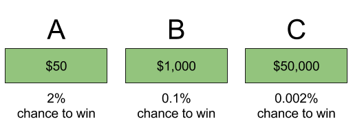
Suppose each ticket costs 50 cents, and you have one million dollars to spend. Crucially, it doesn’t matter which ticket you buy! Each of these tickets has the same expected value: $1. Thus, it doesn’t matter if you spend the million dollars on A, B, or C – each leads to the same amount of profit.
The above tickets have equal expected value, but they do not have equal risk. We call people who prefer choice A risk averse; whereas someone who prefers C is risk seeking.
Introducing Expected Utility
Economic transactions can be difficult to evaluate. When trading an apple for an orange, which is more valuable? That depends on a person’s unique tastes. In other words, value is subjective.
Let utility represent subjective value. We can treat utility as a function u() that operates on objective outcome x. Expected utility, then, is highly analogous to expected value:

Most economists treat utility functions as abstractions: people act as if motivated by a utility function. Neuroeconomic research, however, suggests that utility functions are physically constructed by the brain.
Every person’s utility function may be different. If a person’s utility curve is linear, then expected utility converges onto expected value:

Recall in the above lottery, the behavioral distinction between risk-seeking (preferring ticket A) and risk-averse (preferring C). Well, in practice most people prefer A. Why?
We can explain this behavior by appealing to the shape of the utility curve! Utility concavity produces risk aversion:
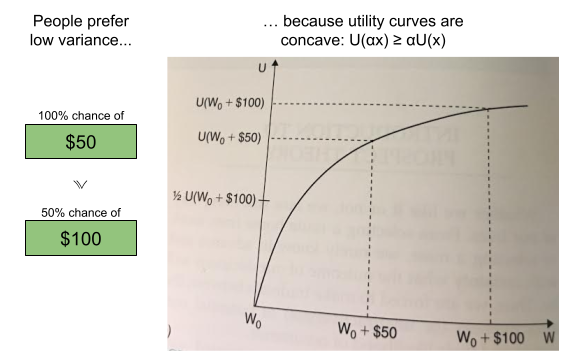
In the above, we see the first $50 (first vertical line) produces more utility (first horizontal line) than the second $50.
Intuitively, the first $50 is needed more than the second $50. The larger your wealth, the less your need. This phenomenon is known as diminishing marginal returns.
Neoclassical Economics
In 1944, von Neumann and Morgenstern formulated a set of axioms that are both necessary and sufficient for representing a decision-maker’s choices by the maximization of expected utility.
Specifically, if you assume an agent’s preference set accommodates these axioms…
1. Completeness. People have preferences over all lotteries.


2. Transitivity. Preferences are expressed consistently.


3. Continuity. Preferences are expressed as probabilities.


4. Substitution. If you prefer (or are indifferent to) lottery 


The above axioms constitute expected utility theory, and form the cornerstone for neoclassical economics. Expected utility theory bills itself as both a normative and descriptive theory: that we understand human decision making, and have a language to explain why it is correct.
Challenges To Substitution Axiom
In the 1970s, expected utility theory came under heavy fire for failing to predict human behavior. The emerging school of behavioral economics gathered empirical evidence that von Neumann-Morgenstern axioms were routinely violated in practice, especially the substitution axiom.
For example, the Allais paradox asks our preferences for the following choices:

Most people prefer A (“certain win”) and D (“bigger number”). But these preferences are inconsistent, because C = 0.01A and D = 0.01B. The substitution axiom instead predicts that A ≽ B if and only if C ≽ D.
The Decoy effect contradicts the Independence of Irrelevant Alternatives (IIA). I find it to be best illustrated with popcorn:

Towards a Value Function
Concurrently to these criticisms of the substitution axiom, the heuristics and biases literature (led by Kahneman and Tversky) began to discover new behaviors that demanded explanation:
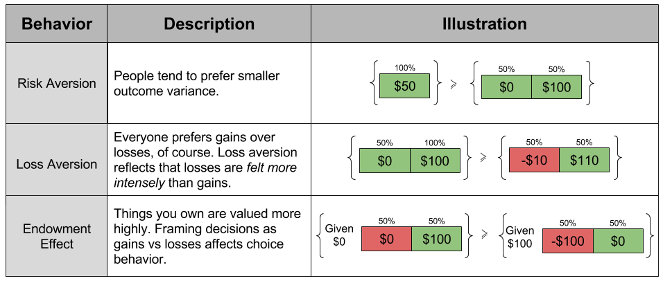
- Risk Aversion. In most decisions, people tend to prefer smaller variance in outcomes.
- Everyone prefers gains over losses, of course. Loss Aversion reflects that losses are felt more intensely than gains of equal magnitude.
- The Endowment Effect. Things you own are intrinsically valued more highly. Framing decisions as gains or as losses affects choice behavior.
Each of these behavioral findings violate the substitution axiom, and cumulatively demanded a new theory. And in 1979, Kahneman and Tversky put forward prospect theory to explain all of the above effects.
Their biggest innovation was to rethink the utility function. Do you recall how neoclassical economics appealed to 
Let value function 


Terminology aside, each theory only differs in the shape of its outcome function.

Let us now look closer at the the shape of 
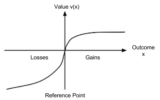
This shape allows us to explain the above behaviors:
The endowment effect captures the fact that we value things we own more highly. The reference point in 
Loss aversion captures the fact that losses are felt more strongly than gains. The magnitude of
We have already explained risk aversion by concavity of the utility function
Towards a Weight Function
Another behavioral discovery, however, immediately put prospect theory in doubt:
- The Fourfold Pattern. For situations that involve very high or very low probabilities, participants often switch their approaches to risk.
To be specific, here are the four situations and their resultant behaviors:
- Fear of Disappointment. With a 95% chance to win $100, most people are risk averse.
- Hope To Avoid Loss. With a 95% chance to lose $100, most people are risk seeking.
- Hope Of Large Gain. With a 5% chance to win $100, most people are risk seeking.
- Fear of Large Loss. With a 5% chance to lose $100, most people are risk averse.
Crucially,

Failed predictions are not a death knell to a theory. Under certain conditions, they can inspire a theory to become stronger!
Prospect theory was improved by incorporating a probability-weighting function.

Where 
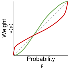
These are in fact two probability-weighting functions (Hertwig & Erev 2009)
- Explicit weights represent probabilities learned through language; e.g., when reading the sentence “there is a 5% chance of reward”.
- Implicit weights represent probabilities learned through experience, e.g., when the last 5 out of 100 trials yielded a reward.
This change adds some mathematical muscle to the ancient proverb:
Humans don’t handle extreme probabilities well.
And indeed, the explicit probability-weighting function successfully recovers the fourfold pattern:

Takeaways
Today we have reviewed theories of expected value, expected utility (neoclassical economics), and prospect theory. Each theory corresponds to a particular set of conceptual commitments, as well a particular formula:
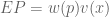
However, we can unify these into a single value formula V:

In this light, EV and EU have the same structure as prospect theory. Prospect theory distinguishes itself by using empirically motivated shapes:

With these tools, prospect theory successfully recovers a wide swathe of economic behaviors.

Until next time.
Works Cited
- Hertwig & Erev (2009). The description–experience gap in risky choice


 , where
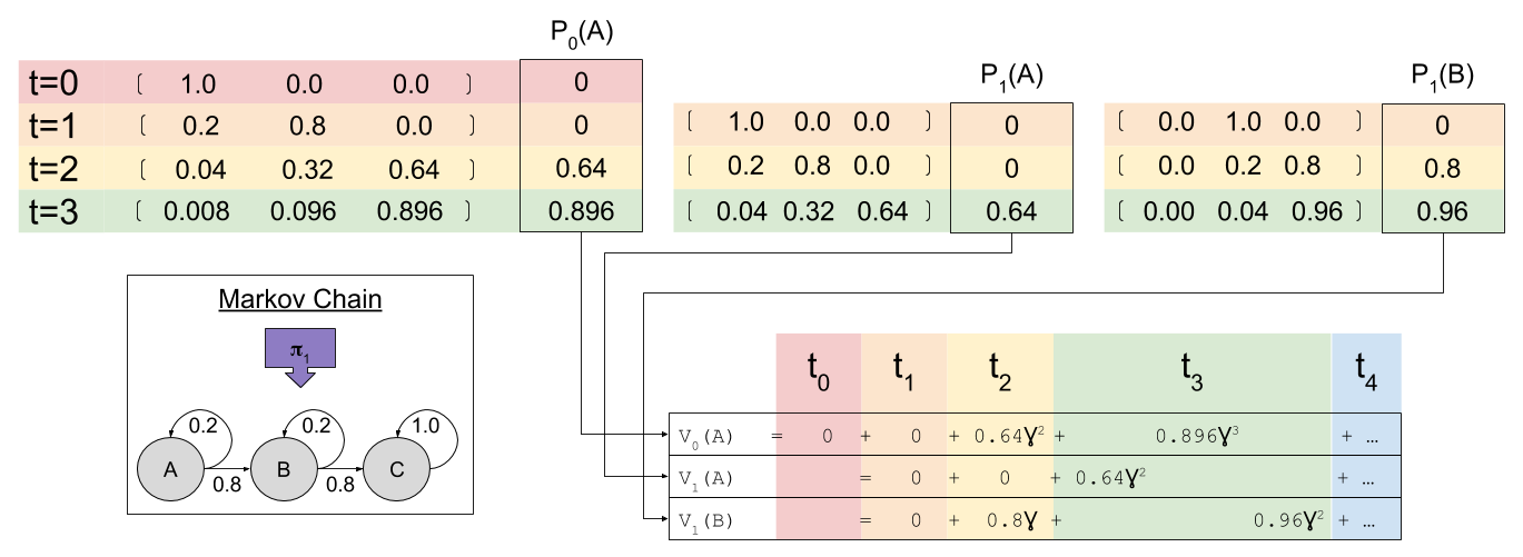
  is the state being considered at the next time step.


 :
:
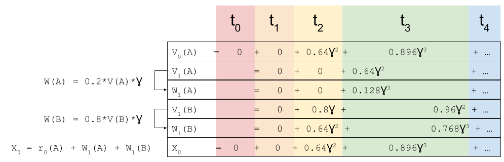
 look familiar? That’s because it equals
  ! In this way, we have a way of equating a valuation at t=0 and t=1. This property is known as intertemporal consistency.
 . Let’
