Part Of: [Advanced Inference In Graphical Models] sequence
Followup To: [Family vs. Universe]

Table Of Contents

• Motivations
• Graph Type: Factor Graphs
• Graph Type: Markov Random Fields
• A Tale Of Three Families
• On Specificity
• Takeaways

Motivations

Today, we’re going to talk through the construction of a family, and how such a construction might succeed or fail.

Across machine learning, there exist dozens of different graph types; of these, three are the most popular:

1. Markov Random Fields
2. Factor Graphs
3. Bayesian Networks

Our example today will span the first two of these graphs.

Graph Type: Markov Random Field

Markov Random Fields (MRFs) have very simple semantics; they are basically undirected graphs:

 

In the above MRF, we have a graph with five vertices and six edges. It’s probability distribution is comprised of three factors, one per maximal clique (the first term corresponds to top-left triangle, etc).

The graphical model of MRFs can be formalized by defining its graph and rule structure. Let us define the following terms:

• Let V represent the set of all vertices in the graph
• Let E represent the set of all edges in the graph

We now define the Markov Random Field:

Here’s how I “translate” all the math on the right:

• “For each cliques in the set of all maximal cliques, there exists a function phi over some collection of variables within the clique.”
• “The joint probability, then, over all variables is the product of all  phi functions in the graph.”

It turns out that there are several other rules which describe an MRF equally well, but maximal-clique factorization rule serves our purposes here well enough.

Introducing Factor Graphs

Factor graphs (FGs) also have undirected edges, but they honor other constraints, as well:

Notice anything interesting about this graph’s edges? […] Did you notice how no v-nodes or f-nodes are never connected one another? In other words, if we group all edges Graphs with this property, that all edges span across two distinct nodesets, are called bipartite graphs.

How is the probability distribution formula constructed? […] On inspection, it becomes clear that each of the four terms on the right-hand side correspond to factor-nodes.

A rigorous definition of factor graphs simply require us to generalize these two observations. First, some vocabulary is in order.

• Let V represents the set of vertex-nodes on the graph (e.g., v₁ through v₃)
• Let F represent the set of factor-nodes on the graph (e.g., f₁ through f₄)
• Let E represent the set of all edges in the graph.

We are now in a position to completely specify the Factor Graph:

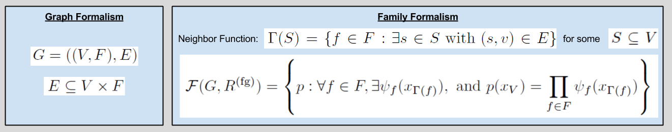
Here’s how I would translate this family definition:

• “Let neighbor function RHO be defined as a function that searches through each factor and returns each neighbor.”
• “For every factor f, there exists a function PSI, which takes as its input all neighbors of f (those neighbors discovered by RHO).”
• “The joint probability is then the product of all such functions PSI.”

 A Tale Of Three Families

Ready to get your hands dirty?! Good! Let’s consider three specific graphs: two factor graphs, and one Markov Random Field:

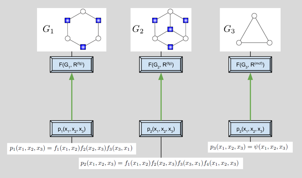
Does this diagram make sense? If not, let me explain each family-distribution pairing in turn.

• The leftmost family represents the semantics of factor-graphs R^(fg), along with a set of factor-nodes, vertex-nodes, and edges G₁. Just as in the factor-graph example above, its corresponding probability distribution is derived from these two elements: each term corresponding to one factor-node and its neighbors.
• The center family is identical to the previous factor-graph, except for an additional factor-node. This additional element corresponds to an extra term in the resultant probability distribution, f₄(…)
• The rightmost family represents the semantics of MRFs (here, maxclique factorization) R^(mcf), along with a set of nodes and edges G₃. Its probability distribution flows from the semantics: since all three variables form a clique, the distribution is a factor across all variables.

So far, so obvious. But recall the purpose of rules: they deliver yes/no answers to any probability distribution that applies for membership. Thus, we must be willing in inquire whether p₁ is a member of Family₂, etc.

Here are the membership results of the six new family applications:

 

A green edge (A, B) means that our Ath distribution is a member of our Bth family. In contrast, a red edge denotes non-membership. Let me explain the results of each new edge in turn:

1. (1,2) is green because f(a, b) -> g(x, y, z) transforms are possible.
2. (1,3) is green because f(a, b) -> g(x, y, z) transforms are possible.
3. (2,1) is red because f(a, b, c) -> g(x, y) transforms are impossible (if they were, they would be expressed as two-term factors originally).
4. (2,3) is green because f(a, b, c) -> g(x, y, z) transforms are possible.
5. (3,1) is red because f(a, b, c) -> g(x, y) transforms are impossible (similar reasoning to (2,1)).
6. (3,2) is green because f(a, b, c) -> g(x, y, z) transforms are possible.

On Specificity & Generality

Consider you find yourself asked to design an graphical model that includes p₁ within its family. As you can see, any of the above graphs satisfy this requirement. But that does not make them equal.

When designing families, we ought to be as narrow as possible. Suppose we don’t particularly care to compute over p₂ or p₃. Then, we have reason to prefer Family₁ asdf – it has the power to say No to these irrelevant distributions, and thereby save computational resources.

Here’s how my professor summarizes & illustrates this principle:

This suggests that there are two aspects of a type of graphical model that indicate its power, and that is: generality, can a graph be found such that its family includes a given distribution; and specificity, how discriminative is a given graph that represents a given distribution.

For example, a collection of all i.i.d. random variables would trivially be a member of all of the aforementioned families, but such a distribution would violate many of the properties that are left unspecied. We might be interested in another graphical model semantics that specifically precludes those cases.

These two notions help us get clear on the kinds of questions to ask when designing a graphical model from scratch.

Takeaways

• When designing a family, one must optimize not just for generality (admitting viable distributions). Specificity (the rejection of irrelevant distributions) matters just as much.