The Reliability Ratio

October 8, 2026kevinbinz 1 Comment

Part Of: Machine Learning sequence
Followup To: OLS Estimation via Projection
Content Summary: 4800 words, 24 min read

The Reliability Ratio

A student scores 2 standard deviations (SD) above the mean on an exam, in about the top 2%. A month later she retakes the exam. Even if nothing about her changes, her second exam score will probably be lower. How much lower? One number answers this question: the reliability ( $λ$ ) of the test.

To understand reliability, classical test theory (CTT) splits her score into two steps. Write it as $x = s + n$ . The first step, the signal s, runs from the population mean to the student’s true score: the average she would earn over many sittings. The second step, the noise n, runs from her true score to her observed score.

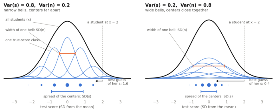
Let’s imagine each true score is a type. Students of the same type still get different scores, because each sitting draws its own error. Suppose type k has true score $s_k$ and makes up a fraction $p_k$ of the population. Each distribution of types is the normal distribution $\mathcal{N}\big(s_k, \operatorname{Var}(n)\big)$ . The population is their weighted sum:

$f(x) = \sum_k p_k , \mathcal{N}\big(s_k, \operatorname{Var}(n)\big)$

The same distribution of observed scores can come from two different situations. One sitting per student cannot tell the two situations apart.

Because n is independent of s, the two variances add:

$\operatorname{Var}(x) = \operatorname{Var}(s) + \operatorname{Var}(n)$

To see why, square a student’s deviation: $(s+n)^2 = s^2 + 2sn + n^2$ . Average each term over all students. The first gives $Var(s)$ , and the last gives $Var(n)$ . Inside one bell, s is fixed and n averages to zero, so the cross term $2sn$ also averages to zero.

Because the variances add, each one is a share of the whole. The share that comes from true scores is the reliability of the test:

$\text{Reliability: } \lambda = \frac{\operatorname{Var}(s)}{\operatorname{Var}(x)}$

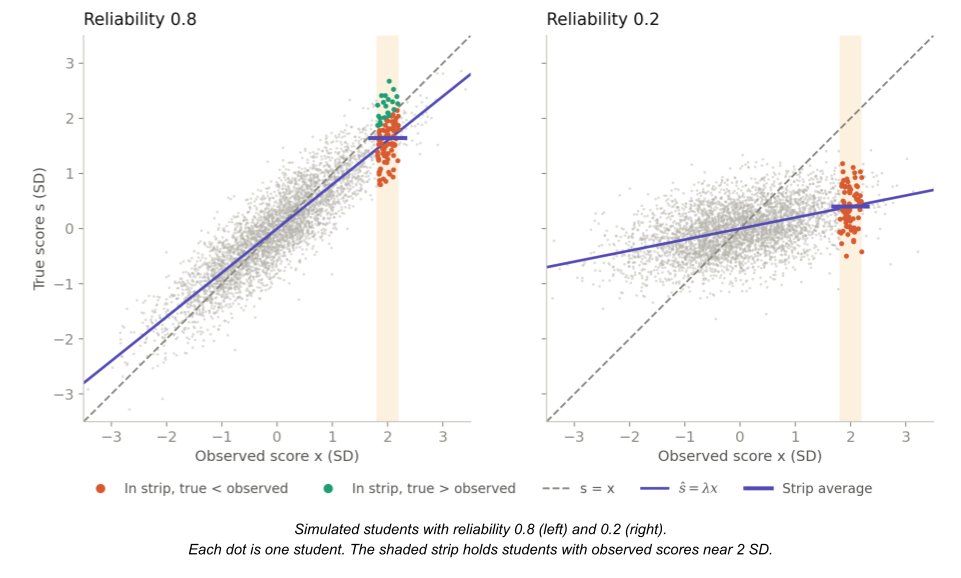
It runs from 0 to 1, and the error share is 1 − λ. In the figure, Var(x) = 1, so λ is 0.8 on the left and 0.2 on the right. So λ describes a test in one population. Give the same test to a narrower population, and Var(s) falls while Var(n) stays the same, so λ falls.

The Coefficient of Determination

Reliability answers a question: how much of the variance in observed scores does the true score predict? Regression answers the same question with the coefficient of determination.

Regress an outcome y on one predictor. The fitted line makes a prediction ŷᵢ for each observation, and the residual $eᵢ = yᵢ − ŷᵢ$ is the error that remains.

A model’s mean squared error (MSE) measures the performance of the model:

$\text{MSE}{\text{model}} = \frac{1}{N}\sum_i (y_i – \hat{y}i)^2 = \frac{1}{N}\sum_i e_i^2$

The coefficient of determination (R²) measures how well the model’s predictions track the outcome. It compares the model’s MSE with a baseline that predicts the mean ȳ for every observation:

$\text{MSE}{\text{base}} = \frac{1}{N}\sum_i (y_i – \bar y)^2 = \operatorname{Var}(y) R^2 = 1 – \frac{\text{MSE}{\text{model}}}{\text{MSE}{\text{base}}}$

If the model predicts every observation exactly, R² = 1. If it matches the baseline, R² = 0.

Two properties of least squares will be used in this section. First, the residuals average to zero. Second, they are uncorrelated with the predictions.

Given the first property, and the fact that a variable with zero mean has a variance equal to its mean square:

$\text{MSE}{\text{model}} = \frac{1}{N}\sum_i e_i^2 = \operatorname{Var}(e).$

We can now write the coefficient of determination in terms of variances:

$R^2 = 1 – \frac{\operatorname{Var}(e)}{\operatorname{Var}(y)} = \frac{\operatorname{Var}(y) – \operatorname{Var}(e)}{\operatorname{Var}(y)}$

The second property splits the variance of the outcome. Since y = ŷ + e, its variance is,

$\operatorname{Var}(\hat y + e) = \operatorname{Var}(\hat y) + \operatorname{Var}(e) + 2\operatorname{Cov}(\hat y, e)$

The covariance term is zero, so

$\operatorname{Var}(y) = \operatorname{Var}(\hat y) + \operatorname{Var}(e)$

Substitute this into the numerator:

$R^2 = \frac{\operatorname{Var}(\hat y)}{\operatorname{Var}(y)}$

This equation is why R² is also called the explained variance.

In CTT, the noise n has both properties, so x = s + n is a least-squares regression with fit x̂ = s. We cannot run this regression, because true scores are hidden. Its R² still exists, and it is the reliability:

$R^2 = \frac{\operatorname{Var}(\hat x)}{\operatorname{Var}(x)} = \frac{\operatorname{Var}(s)}{\operatorname{Var}(x)} = \lambda$

CTT assumes these properties. In regression, least squares provides them for the training data. On new data, the model can underperform baseline, and R² can be negative.

The Geometry of Variance

OLS Estimation via Projection showed that least squares projects a vector onto the column space of a matrix A. The residual e is perpendicular to that space: $A^\top e = 0$ . The same geometry organizes variance.

Treat each variable as a vector with one entry for each of the N students. Subtract the mean from each entry, and divide each entry by √N. The covariance is an average of products:

$\operatorname{Cov}(u, v) = \frac{1}{N}\sum_{i=1}^{N} (u_i – \bar u)(v_i – \bar v)$

Each vector carries a factor of 1/√N, so their dot product carries 1/N. For these vectors, statistics and geometry are related by the following identities.

$\operatorname{Cov}(u, v) = u \cdot v, \qquad \operatorname{Var}(u) = |u|^2, \qquad \sigma_u = |u|$

The correlation (r) of two variables is the covariance of their standardized versions, $z_u = u/\sigma_u$ and $z_v = v/\sigma_v$ . In vector terms, this divides the dot product by both lengths, which gives the cosine of the angle between the vectors:

$\text{Correlation: } r = \frac{\operatorname{Cov}(u, v)}{\sigma_u \sigma_v} = \operatorname{Cov}(z_u, z_v) = \frac{u \cdot v}{|u|,|v|} = \cos\theta$

Two uncorrelated variables have r = 0 = cos 90°, so they are perpendicular.

Signal and noise are uncorrelated, so they are perpendicular, and $x = s + n$ is the hypotenuse of a right triangle. The legs have lengths $\sigma_s = 4$ and $\sigma_n = 3$ , and the hypotenuse has length $\sigma_x = 5$ . The lengths do not add: 4 + 3 ≠ 5. The areas of the squares on the sides are the variances, and they do add: 16 + 9 = 25. In this geometry, variance additivity is the Pythagorean theorem. Fisher (1918) introduced the term variance because of this additivity.

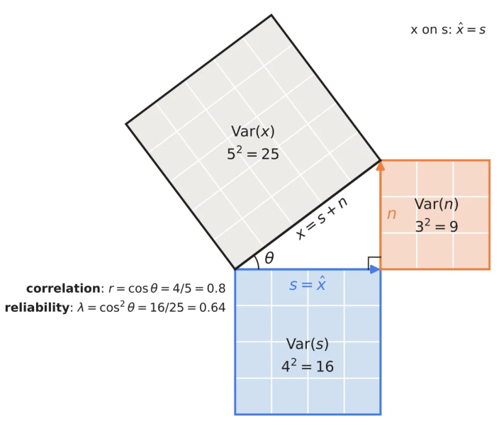
The split $Var(y) = Var(ŷ) + Var(e)$ in the previous section is the same theorem. The prediction and the residual are uncorrelated, so they are perpendicular. Because the vectors are centered, a regression on one predictor projects the outcome onto the predictor.

For an outcome v and a predictor u, the residual $v − bu$ is perpendicular to u, so $u · (v − bu) = 0$ . Write $b_{v|u}$ for the slope of v on u.

$b_{v|u} = \frac{u \cdot v}{u \cdot u} = \frac{\operatorname{Cov}(u, v)}{\operatorname{Var}(u)}$

The slope is the covariance of the predictor and the outcome, divided by the variance of the predictor. The triangle shows the regression of x on s from the previous section. The residual n is perpendicular to the predictor s, so the fit is s itself, and b_{x|s} = 1.

The side s is adjacent to the angle θ, and x is the hypotenuse, so

$r = \cos\theta = \frac{|s|}{|x|} = \frac{\sigma_s}{\sigma_x} = \frac{4}{5} = 0.8$

$\lambda = R^2 = \frac{|s|^2}{|x|^2} = \cos^2\theta = r^2 = \frac{16}{25} = 0.64$

The reliability is the squared correlation between true and observed scores. This holds for any regression with one predictor:

$R^2 = \cos^2\theta = r^2$

Regression to the Mean

The slope of y on x is $Cov(x, y)/Var(x)$ . Measure both variables in standard deviations, and the slope becomes r. The slope of x on y is also r. In any units, the two slopes multiply to r²:

$b_{y|x}, b_{x|y} = \frac{\operatorname{Cov}(x,y)}{\operatorname{Var}(x)} \cdot \frac{\operatorname{Cov}(x,y)}{\operatorname{Var}(y)} = r^2$

In standard units, unless the correlation is exact, every prediction is less extreme than its predictor. Galton (1886) found this in human stature. He compared the heights of children with the mean height of their parents and found a slope of about two thirds: parents whose mean height is 3 inches above average have children about 2 inches above average. He called this effect regression towards mediocrity. We now call it regression to the mean.

The slope of about two thirds is measured in inches per inch. It differs from the correlation because parental averages vary less than children’s heights.

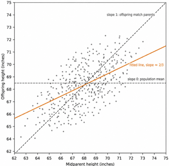
Regression to the mean also runs backward in time: tall children have parents who are, on average, less tall than they are. The effect doesn’t require a causal mechanism. It manifests whenever measurements share a signal but also draw independent noise.

When a test is administered twice, for example, the two sittings share a true score and nothing else, so their covariance is Var(s). They also have the same variance, Var(x). So the slope of retest on test and their correlation are both $Var(s)/Var(x) = λ$ .

Galton’s data has the same structure. The mid-parent height is a noisy measure of the parents’ mean additive genetic value: the part of genetic value that children inherit on average. A child inherits that value and draws new noise of its own. So the covariance of child and mid-parent is the variance of the genetic signal, and the slope of child on mid-parent is a reliability ratio. The child’s height varies more than the mid-parent’s, so here only the slope equals this ratio. Quantitative genetics calls this ratio heritability. Under simple genetic assumptions, Galton’s slope of about two thirds measures the heritability of height.

Reliability is the slope of retest on test. It is the component of a result that carries over to the next measurement.

Shrinkage

Recall our student with a strong test score. Regression to the mean says her retest will probably be lower. What is her true score?
The geometry section knew the true score (s) and predicted the observed score (x). It regressed x on s. Our student’s case runs the other way. We know only her observed score, so we regress s on x to estimate her true score.

Independent noise adds nothing to a covariance, so the covariance of the true and observed scores is the variance of the signal:
$\operatorname{Cov}(s, x) = \operatorname{Var}(s)$

A slope is this covariance divided by the variance of the predictor, so only the denominator changes:

$b_{x|s} = \frac{\operatorname{Var}(s)}{\operatorname{Var}(s)} = 1, \qquad b_{s|x} = \frac{\operatorname{Var}(s)}{\operatorname{Var}(x)} = \lambda$

If we know a student’s true score, her observed score averages to that true score. When true scores and errors are normal, no curve does better than the line ŝ = λx. This estimate is called Kelley’s rule. Kelley (1927) derived it in the context of test scores. It is a weighted average of the test score X and the population mean μ:

$\hat{s}_{\text{raw}} = \lambda X + (1-\lambda)\mu$

If the test has high reliability, the estimator trusts the score. Else, it trusts the population mean.

Consider students who achieve a test score of 2 SD. By definition of the normal distribution, many of these students have a true score near 1 SD. So an observed score of 2 SD comes more often from a good student with good luck than from an excellent student with average luck. Consider one of these students. Reliability tells us how much of her lead is skill. With a reliability of 0.8, about 80% of her 2 SD lead is skill, so her best-guess true score is about 1.6 SD.

A Kalman filter (Kalman 1960) tracks a hidden quantity with a current estimate. The estimate’s error has variance P, and each measurement adds noise with variance R. These play the same roles of Var(s) and Var(n) in CTT. The estimate has variance P + R. The filter moves its estimate toward the measurement by a weight K called the gain:

$K = \frac{\operatorname{Var}(\text{true step})}{\operatorname{Var}(\text{measured step})} = \frac{P}{P + R}$

The Kalman filter uses Kelley’s rule, but with the current estimate in place of the population mean. A noisy measurement has a small gain and is largely ignored.

Reliability is also a shrinkage factor. It is the share of an observed lead that we credit to the true score.

Attenuated Slopes

The true scores are often latent, but estimating them can enable downstream predictions. An epidemiologist wants to know how much stroke risk rises with blood pressure. She needs the slope of stroke risk y on each patient’s usual blood pressure s. But she has only one reading x per patient, a noisy measure of s. If she regresses stroke risk on the readings, what slope does she get?

Suppose an outcome depends on the true score, $y = βs + ε$ . The slope we want is $b_{y|s} = \beta$ . True scores are hidden, so we can fit only $b_{y|x}$ , the regression of y on the observed score x = s + n. Write $\lambda_x$ for the reliability of x.

$x = s + n,\quad y = \beta s + \varepsilon,\quad b_{y|x} = \frac{\operatorname{Cov}(y,\ x)}{\operatorname{Var}(x)} = \frac{\operatorname{Cov}(\beta s + \varepsilon,\ s + n)}{\operatorname{Var}(x)}$

If we assume the noise n and the error ε are independent of s and of each other, they add nothing to the covariance:

$\operatorname{Cov}(\beta s + \varepsilon,\ s + n) = \beta\operatorname{Var}(s) + \beta\operatorname{Cov}(s, n) + \operatorname{Cov}(\varepsilon, s) + \operatorname{Cov}(\varepsilon, n) = \beta\operatorname{Var}(s)$

$b_{y|x} = \frac{\operatorname{Cov}(\beta s + \varepsilon,\ s + n)}{\operatorname{Var}(x)} = \beta,\frac{\operatorname{Var}(s)}{\operatorname{Var}(x)} = b_{y|s}, b_{s|x} = \beta\lambda_x$

The slope from a noisy predictor is a product of two factors. The first shrinks the observed score to estimated true score by the reliability. The second factor β carries the true score to the outcome. This process is known as attenuation bias, or regression dilution.

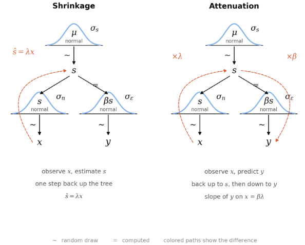
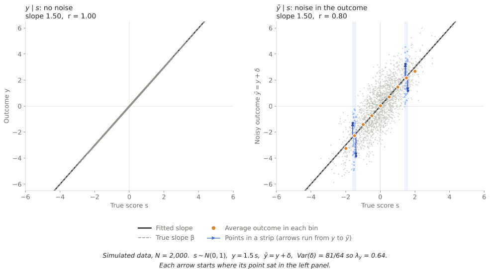
An illustration of the shrinkage. Adding noise to the predictor is visualized as horizontal arrows. The slope of the estimated function flattens.

Her slope from the readings is $\beta\lambda_x$ . For predicting stroke from one reading, this is the best slope she can use. To recover β itself, she divides her slope by $\lambda_x$ , which she can estimate from repeated readings on some of her patients. MacMahon et al. (1990) made this correction in studies of blood pressure and heart disease. The corrected associations with stroke and coronary heart disease were about 60% stronger than the uncorrected ones.

A related effect appears in models trained on many features. Suppose the model also sees a feature z that correlates with the true score s. Then z takes over part of the weight that x loses, even if z has no effect on the outcome. If s is a confounder, epidemiologists call the bias that remains after adjusting for x residual confounding (Phillips & Davey Smith 1991).

Attenuated Correlations

Suppose we score a model against labels from one radiologist. The labels are a noisy measure of the true outcome. Write the radiologist’s label as

$\tilde{y} = y + \delta$

where δ is the radiologist’s error, independent of s, n, and ε. How does label noise change the slope and the correlation?

In the algebra, δ adds nothing to the covariance, so the slope is unchanged:

$b_{\tilde y|x} = \frac{\operatorname{Cov}(y + \delta,\ x)}{\operatorname{Var}(x)} = \frac{\operatorname{Cov}(y,\ x)}{\operatorname{Var}(x)} = b_{y|x}$

But the noisy label does attenuate the correlation. Recall our definitions.

$r_{\text{true}} = \frac{\operatorname{Cov}(s,\ y)}{\sigma_s,\sigma_y}, \qquad r_{\text{observed}} = \frac{\operatorname{Cov}(x,\ \tilde y)}{\sigma_x,\sigma_{\tilde y}}$

\lambda_x = \frac{\mathrm{Var}(s)}{\mathrm{Var}(x)}, \qquad \sqrt{\lambda_x} = \frac{\sigma_s}{\sigma_x}, \qquad \lambda_y = \frac{\mathrm{Var}(y)}{\mathrm{Var}(\tilde{y})}, \qquad \sqrt{\lambda_y} = \frac{\sigma_y}{\sigma_{\tilde y}}

The noises are independent, so the numerators are equal.

$\operatorname{Cov}(x,\ \tilde y) = \operatorname{Cov}(s + n,\ y + \delta) = \operatorname{Cov}(s,\ y)$

Multiply the true correlation by a ratio of standard deviations to get the observed correlation:

r_{\text{true}} \frac{\sigma_s \sigma_y}{\sigma_x \sigma_{\tilde y}} = \frac{\mathrm{Cov}(s, y)}{\sigma_s \sigma_y} \cdot \frac{\sigma_s \sigma_y}{\sigma_x \sigma_{\tilde y}} = \frac{\mathrm{Cov}(x, \tilde y)}{\sigma_x \sigma_{\tilde y}} = r_{\text{observed}}

Both reliability ratios reduce the correlation, so observed correlations are closer to zero than true correlations.

r_{\text{observed}} = r_{\text{true}} \frac{\sigma_s}{\sigma_x} \frac{\sigma_y}{\sigma_{\tilde y}} = r_{\text{true}} {(\lambda_x \lambda_y}^{1/2})

Spearman (1904) named this weakening attenuation. To correct an observed correlation, divide it by $(\lambda_x \lambda_y)^{1/2}$ .

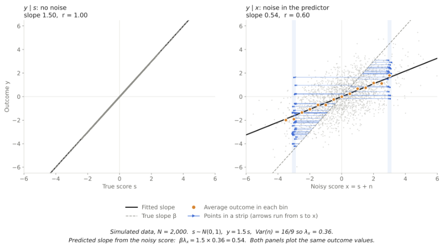
In the figure, the left panel has no noise. In the right panel, each point moves up or down by its noise, and its true score stays the same. The noise averages to zero in each bin, so the orange dots stay on the true line, and the slope stays at 1.5. The correlation falls from 1 to ${\lambda_y}^{1/2} = 0.8$ .

These are the regressions of this post, each with its slope and correlation.

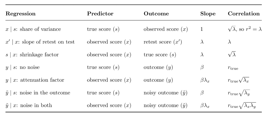
Reliability is also an attenuation factor. A noisy predictor keeps the share λ of a true slope, and each noisy measurement keeps the share √λ of a true correlation.

Estimating Reliability

So far, we have treated the reliability λ as known. In practice, we must estimate it. One score per student cannot provide an estimate, but a second score of the same student can. Since test and retest share the true score and nothing else, we saw that their correlation was λ. More sittings give a better estimate of λ, and their average is a more reliable score.

Suppose each of N students sits the test m times. The score of student i on sitting j, and her average across all sittings are:

$x_{ij} = s_i + n_{ij}, \qquad \bar{x}_i = s_i + \bar{n}_i$

The true score and the errors are independent, so their variances add

$\operatorname{Var}(\bar{x}_i) = \operatorname{Var}(s) + \operatorname{Var}(\bar{n}_i) = \operatorname{Var}(s) + \frac{\operatorname{Var}(n)}{m}$

Across m sittings, the reliability of the average $\lambda_m$ is the share of this variance that comes from the true score.

$\lambda_m = \frac{\operatorname{Var}(s)}{\operatorname{Var}(\bar{x}_i)} = \frac{\operatorname{Var}(s)}{\operatorname{Var}(s) + \operatorname{Var}(n)/m}$

For one sitting, recall the signal share and error share:

$\lambda = \frac{\operatorname{Var}(s)}{\operatorname{Var}(x)} \qquad 1-\lambda = \frac{\operatorname{Var}(n)}{\operatorname{Var}(x)}$

The relationship between reliability of the average and single-sitting reliability is known as the Spearman-Brown formula (Spearman 1910; Brown 1910).

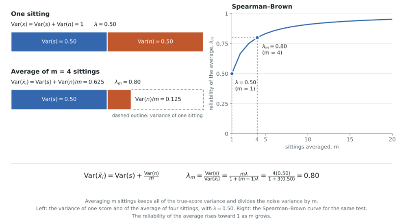
$\lambda_m = \frac{m\lambda}{1 + (m-1)\lambda}$

Repeated sittings also let us estimate the signal and noise variances. The spread of each student’s scores around her own average estimates Var(n). The spread of the student averages around the grand average x̄, the average of all the scores, estimates Var(x̄ᵢ):

$\widehat{\operatorname{Var}}(n) = \frac{1}{N(m-1)}\sum_{i=1}^{N}\sum_{j=1}^{m}\left(x_{ij}-\bar{x}_i\right)^2 \qquad \widehat{\operatorname{Var}}(\bar{x}i) = \frac{1}{N-1}\sum{i=1}^{N}\left(\bar{x}_i-\bar{x}\right)^2$

These divisors differ from the 1/N of earlier sections. Scores sit closer to their own average than to their true mean, so dividing by the number of scores would give too small an estimate. Each divisor counts degrees of freedom: m – 1 inside each of the N students, and N – 1 for the averages.

Replace each variance in the equation for the variance of the average with its estimate, solve for the signal variance, and substitute the estimates into both reliabilities:

$\widehat{\operatorname{Var}}(s) = \widehat{\operatorname{Var}}(\bar{x}_i) – \frac{\widehat{\operatorname{Var}}(n)}{m} \qquad \hat{\lambda} = \frac{\widehat{\operatorname{Var}}(s)}{\widehat{\operatorname{Var}}(s) + \widehat{\operatorname{Var}}(n)} \qquad \hat{\lambda}_m = \frac{\widehat{\operatorname{Var}}(s)}{\widehat{\operatorname{Var}}(s) + \widehat{\operatorname{Var}}(n)/m}$

Thus, the Spearman–Brown formula can be applied to estimate λ and $\lambda_m$ .

This method is the analysis of variance (ANOVA), and Hoyt (1941) used it to estimate reliability. ANOVA states both spreads on the scale of one sitting, as the mean square within (MSW) and the mean square between (MSB).

$\text{MSW} = \widehat{\operatorname{Var}}(n) \qquad \text{MSB} = m,\widehat{\operatorname{Var}}(\bar{x}_i)$

More sittings make the noise estimate precise. Only more students make the signal estimate precise, because the spread of the averages has N-1 degrees of freedom.

A retest needs a second sitting. Cronbach’s alpha (Cronbach 1951) estimates reliability from one sitting. Each question acts as a short retest of the same true score. So each covariance between two questions estimates the signal variance, and each question’s variance estimates the variance of one score. The average covariance c over the average variance v then estimates the reliability of one question. This estimate assumes that every question measures the true score equally strongly. The m questions play the role of m sittings, and the total score has the same reliability as their average. So the Spearman–Brown formula gives alpha:

$\alpha = \frac{m,c/v}{1 + (m-1),c/v} = \frac{m,c}{v + (m-1),c}$

Psychometricians use alpha to build tests: they keep the questions that raise alpha and drop the ones that lower it.

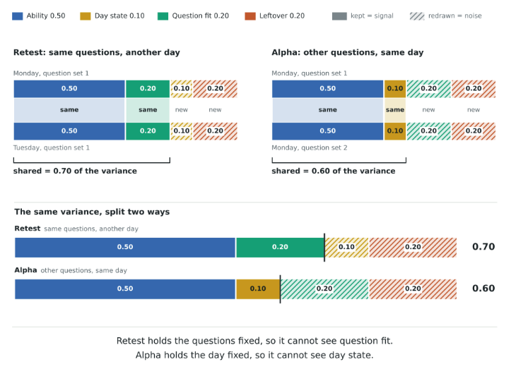
The two formulas average over different replications. For reliability of the average, the replications are m sittings of the same test on different days. For alpha, they are the m questions of one sitting. Retest reliability and Cronbach’s alpha can differ for the same test. A more granular analysis of variance explains the divergence. Divide each score into four parts:

Ability (e.g., intelligence)
Day state (e.g., sleep or mood)
Question fit (e.g., having studied these topics)
Leftover (e.g., a lucky guess)

Administering a test again on a different day keeps only ability and question fit. Administering different questions in one sitting retains ability and day state. This approach to variance is further elaborated in generalizability theory (Cronbach et al. 1972).

Hierarchical Models

CTT has two levels: students taking multiple tests (i.e., sittings). A hierarchical model (HM) has two levels, but at a different granularity: groups having multiple members. In HM, each score is an observation of the group mean. Sittings are glossed over as part of the individual variance.

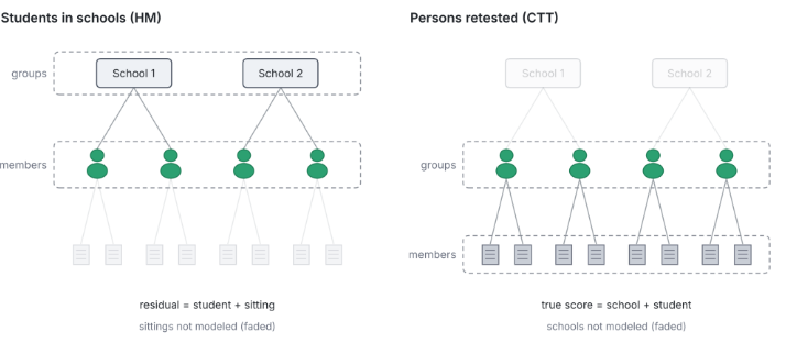
Many of our CTT constructs reappear in HM with new labels.

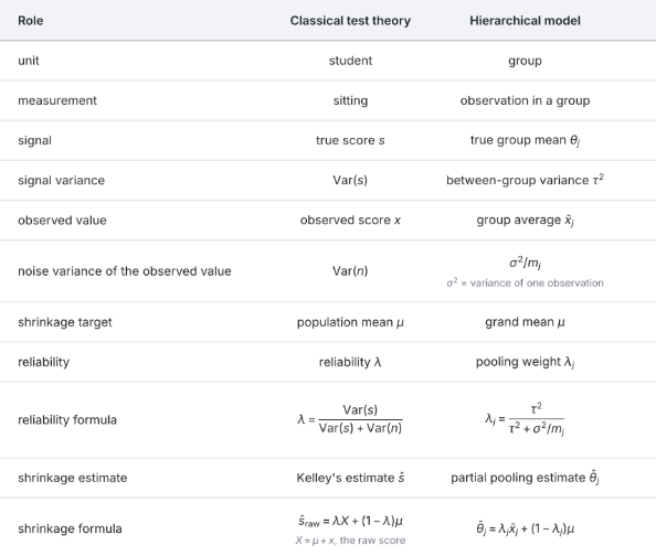
CTT gives every student the same number of sittings, but HM lets groups differ in size. Let mⱼ be the number of students in school j. A school with 20 students and a school with 2,000 students might each report average test scores, and the score of the former is much noisier. Let τ² denote the variance of the true group scores, and σ² denote the variance of student scores within the school. The Spearman–Brown formula gives the reliability of each school:

$\lambda_j = \frac{\tau^2}{\tau^2 + \sigma^2/m_j}$

The estimate of each group mean is Kelley’s rule, with the grand mean μ in place of the population mean:

$\hat{\theta}_j = \lambda_j,\bar{x}_j + (1-\lambda_j),\mu$

Statisticians call this estimate partial pooling. It is a compromise between no pooling (each school keeps its own score) and complete pooling (every group is estimated with the grand mean). Each estimate θ̂ⱼ depends on τ², σ², and μ, and all three come from every group. So each estimate uses information from the other groups. This is known as borrowing strength.

With equal sizes, one weight scales every average, and the rank order stays the same. With unequal sizes, small groups move further toward the grand mean than large groups, so groups can change rank. Wainer (2007) described a case from education. Small schools were overrepresented among the schools with the highest test scores, and this result encouraged large investments in smaller schools. Small schools were also overrepresented among the schools with the lowest scores.

Wainer named the rule behind this pattern de Moivre’s equation: the error of an average of m observations has standard deviation σ/√m. A small school averages few students, so its average has a large error. Large errors put small schools in both tails. The same rule puts small units in both tails in other domains. The US counties with the highest and the lowest kidney cancer death rates are mostly small rural counties (Gelman & Price 1999). Hospitals that treat few patients have the most extreme death rates (Spiegelhalter 2005). Products with few reviews fill both ends of rating lists. Partial pooling moves these small units toward the grand mean.

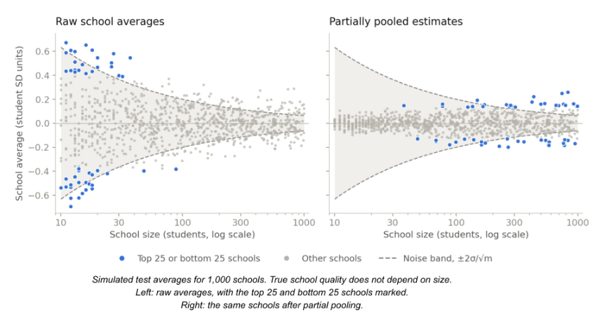
In the left panel, all 50 of the most extreme schools have fewer than 100 students. In the right panel, the extremes are now mostly large schools.

Reliability is also a pooling weight. It is the share of its own average that each group keeps.

Reliability and Regularization

Intro to Regularization added a penalty on the size of a model’s weights. With standardized and uncorrelated features, this ridge penalty shrinks each least-squares weight toward zero by a factor with the same form as the reliability ratio (Hastie et al. 2009). An unregularized fit corresponds to perfect reliability, taking the data at face value. Training on inputs with added noise has the same effect as ridge regression for linear models (Bishop 1995), so attenuation is also a form of regularization.

Maximum likelihood estimation (MLE) estimates each mean by its observed value. But noise accumulates, and the estimate vector is too long on average. Stein (1956) showed that for three or more means, the MLE is inadmissible: another estimator has lower expected total squared error for every possible set of true means. The means can be unrelated, which is why the result is called Stein’s paradox. James & Stein (1961) gave such an estimator. It pulls every estimate toward zero by one shared reliability factor: the share of the estimates’ squared size that comes from the true means.

Model selection compares candidate models and keeps the one with the best score. Any score used to make this choice is optimistic. The winner probably had good luck on the scoring data, and its score will probably decrease on fresh data. This phenomenon of selection bias (Cawley & Talbot 2010) is another form of regression to the mean. Bidders in auctions call it the winner’s curse (Capen et al. 1971). Data partitioning creates a retest. An untouched holdout set draws fresh luck, so its score is honest.

Wrapping Up

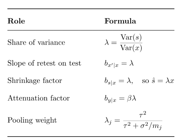
The reliability λ plays five roles:

References

Bishop (1995). Training with noise is equivalent to Tikhonov regularization.
Brown (1910). Some experimental results in the correlation of mental abilities.
Capen, Clapp & Campbell (1971). Competitive bidding in high-risk situations.
Cawley & Talbot (2010). On over-fitting in model selection and subsequent selection bias in performance evaluation.
Cronbach (1951). Coefficient alpha and the internal structure of tests.
Cronbach et al. (1972). The Dependability of Behavioral Measurements.
Fisher (1918). The correlation between relatives on the supposition of Mendelian inheritance.
Galton (1886). Regression towards mediocrity in hereditary stature.
Gelman & Price (1999). All maps of parameter estimates are misleading.
Hastie, Tibshirani & Friedman (2009). The Elements of Statistical Learning.
Hoyt (1941). Test reliability estimated by analysis of variance.
James & Stein (1961). Estimation with quadratic loss.
Kalman (1960). A new approach to linear filtering and prediction problems.
Kelley (1927). Interpretation of Educational Measurements.
MacMahon et al. (1990). Blood pressure, stroke, and coronary heart disease. Part 1, prolonged differences in blood pressure: prospective observational studies corrected for the regression dilution bias.
Phillips & Davey Smith (1991). How independent are “independent” effects? Relative risk estimation when correlated exposures are measured imprecisely.
Spearman (1904). The proof and measurement of association between two things.
Spearman (1910). Correlation calculated from faulty data.
Spiegelhalter (2005). Funnel plots for comparing institutional performance.
Stein (1956). Inadmissibility of the usual estimator for the mean of a multivariate normal distribution.
Wainer (2007). The most dangerous equation.

A Portrait of LUCA

April 11, 2026April 11, 2026kevinbinz 1 Comment

Part Of: Biology sequence
Content Summary: 3000 words, 15 min read

The Basic Facts of Abiogenesis

From the geochemistry of the early Earth, life emerged. The abiogenesis phenomenon is interesting in at least two contexts:

First, it is one of the most difficult unsolved scientific problems in the 21st century. Common descent describes how all of the marvelous diversity of biology stem from a single source: a single celled organism called the Last Universal Common Ancestor (LUCA). We have a clear mechanistic understanding for how this complexification was possible: evolution by natural selection.

But natural selection relies on the machinery of genetic inheritance to produce complexity. How was it possible to create the sophisticated nanomachinery of LUCA (e.g., ATP synthase) before natural selection took effect? What other process besides natural selection can produce complexification?

Second, abiogenesis research is relevant to questions in astrobiology:

Could extraterrestrial life have begun much earlier?

Gen 1 stars (born 13.5-13 Ga) had no exoplanets because the heavy elements required for planetary cores didn’t exist (supernova nucleosynthesis arrived later).
Gen 2 stars (born 13-10 Ga) may have been able to support life, but these exoplanets were small, terrestrial, and less metallic – unable to furnish geomagnetism nor plate tectonics.
Gen 3 stars (born 10-0 Ga) can support life. Exoplanets in this era now include gas giants, and are highly metallic. Geomagnetism protects us from UV radiation, and plate tectonics promote mineral diversity.

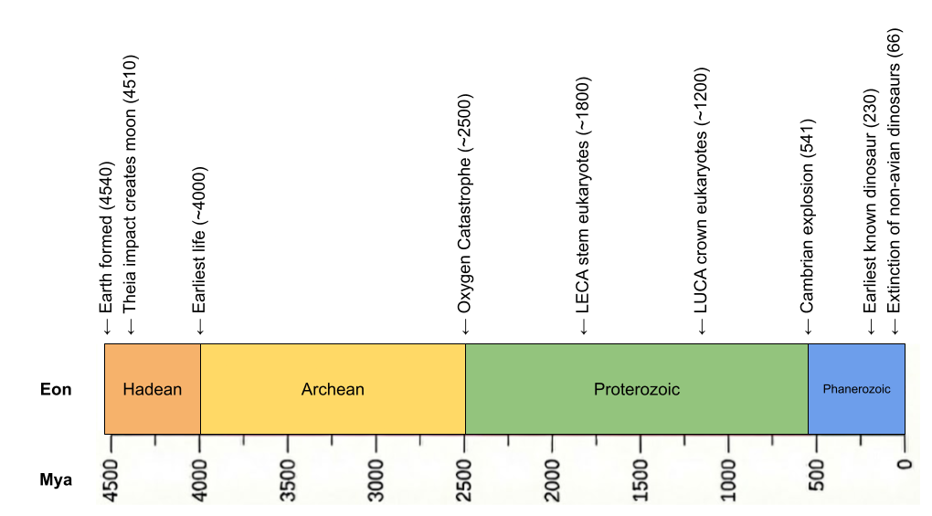
Is abiogenesis easy or hard? The Earth was born 4.6 Ga, with the Theia impactor at 4.54 Ga creating the moon and the Moneta impactor at 4.51 Ga providing siderophilic veneer. Despite such impacts, zircon evidence now suggests a cool early earth, with oceans appearing as early as 4.4 Ga. Critically, our evidence for life arrives very early (Isua banded-iron formations at 3.8 Ga, enriched carbon-12 in zircon graphite at 4.1 Ga). Abiogenesis occurred only ~500 million years after the sterilizing impact of Moneta! Speed is evidence of ease.

If the universe has billions of potentially habitable planets, why haven’t we found any aliens? One explanation to the Fermi Paradox is the Great Filter – some incredibly difficult barrier that prevents life from becoming spacefaring. The scary part is we don’t know where this filter is: behind us (we got incredibly lucky to make it this far) or ahead of us (something typically destroys civilizations before they can spread across the galaxy). If abiogenesis is indeed easy, this might mean the Great Filter is ahead of us.

LUCA from Paleobiogeography

To understand the journey of abiogenesis, we must first understand the destination. What do we know about LUCA?

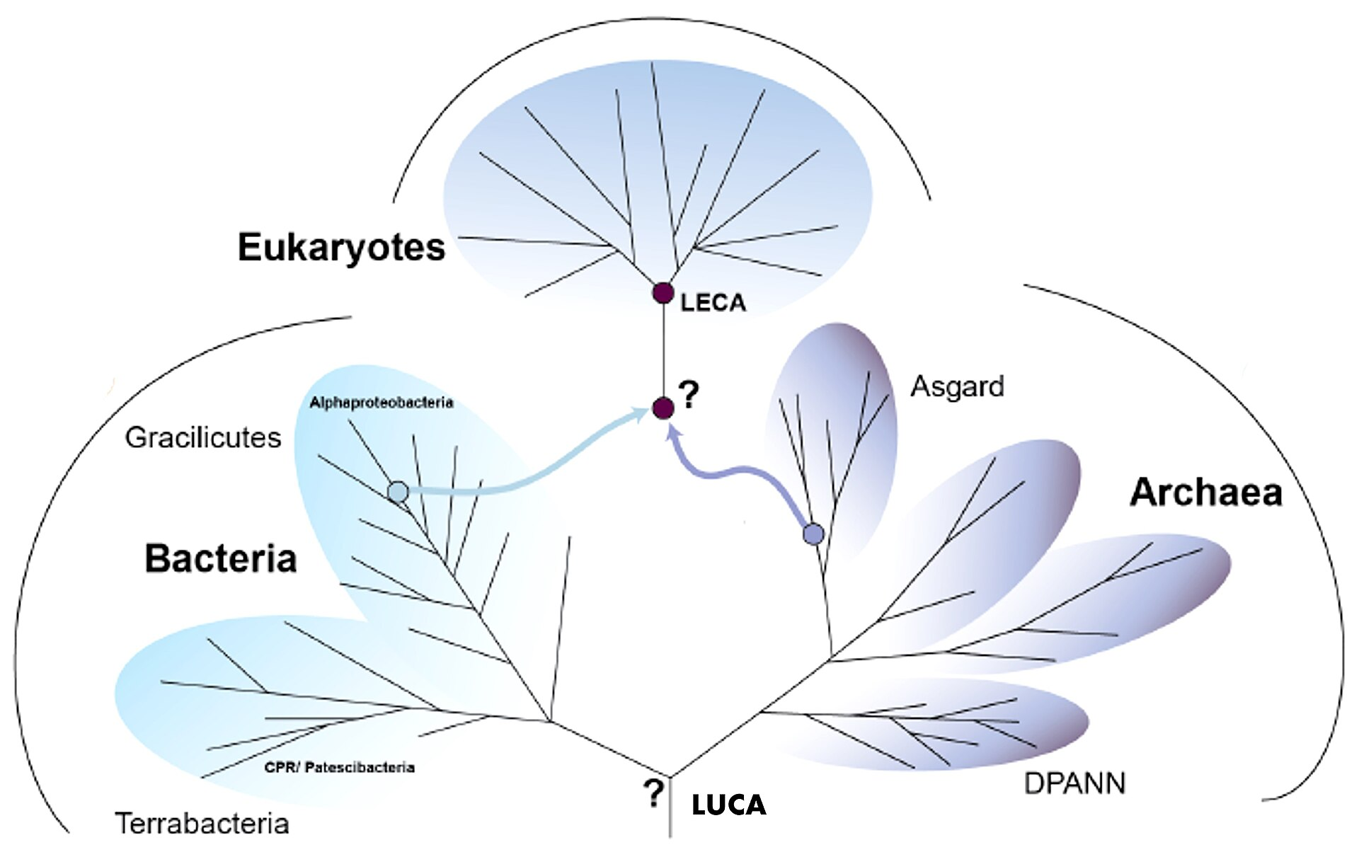
The history of life constrains our search. Two domains of simple life (prokaryotes) emerged in the Hadean: bacteria and archaea. But eukaryotes (complex life) emerged much later, as a result of endosymbiosis between the two families.

Life was microbial for the first 80% of Earth’s history. But in 1.0 Ga, multicellularity was invented. Starting at that time, multicellularity was invented multiple times, but it only really took off in crown group eukaryotes.

LUCA must have been anaerobic. For the first half of Earth’s history, oxygen was locked in water and rocks – there was no free oxygen in the atmosphere. Only when photosynthesis caused the Oxygen Catastrophe in 2.4 Ga did atmospheric oxygen go from 0 to 10%.

LUCA is simple (prokaryotic), microbial (unicellular), and anaerobic.

LUCA from Phylogenetics

We can learn more about LUCA from genetic analyses.

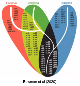
Genes conserved across all species constitute what is called the Universal Gene Set of Life (UGSL), and consists of less than 100 genes (Harris et al 2003). Not surprisingly, the UGSL is dominated by translation-related genes. Here are those ribosomal genes in black:

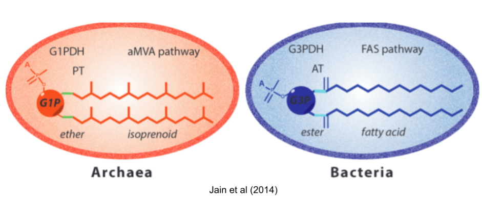
Many differences between archaea and bacteria arose after they diverged. But some differences are more troubling. First among these is the Lipid Divide. Both domains build cells with the phospholipid bilayer membranes, so it is natural to suspect that LUCA had a similar coat. But almost all biochemical details are mirrored! They use different glycerol backbones, different hydrophobic chains (isoprenoid vs fatty acids), different links to those chains (ether vs ester), and different biosynthetic pathways (FAS+AT vs aMVA+PT).

There are three major theories for the lipid composition of LUCA:

Heterochiral theories. LUCA had both lipid biochemistries available. Heterochiral membranes were recently found to be viable (Caforio et al 2018).
Thermoreduction theories. Many archaea are adapted to extreme environments. So LUCA had a bacterial phospholipid, and the more robust archaeal lipids were derived to support more extreme niches.
Protocompartment theories. LUCA didn’t use phospholipids at all! It used a simple fatty acid membrane, or coacervate droplets, or mineral pores to achieve compartmentalization.

Another divergence is even more troubling: bacteria and archaea use completely different DNA replicase proteins (Forterre et al 2013).

Neither divide has a satisfying resolution. Each of the three lipid hypotheses faces serious objections, and the DNA replicase situation is arguably worse: there is no consensus account for how two non-homologous replication machineries could descend from a single ancestor, which has led some (e.g., Forterre 2006) to argue that DNA itself was a viral invention acquired independently by the bacterial and archaeal lineages. Any portrait of LUCA that papers over these divides is overconfident.

LUCA from Biochemistry

At the atomic level, organisms are built with CHNOPS: Carbon, Hydrogen, Nitrogen, Oxygen, Phosphorous, and Sulfur.

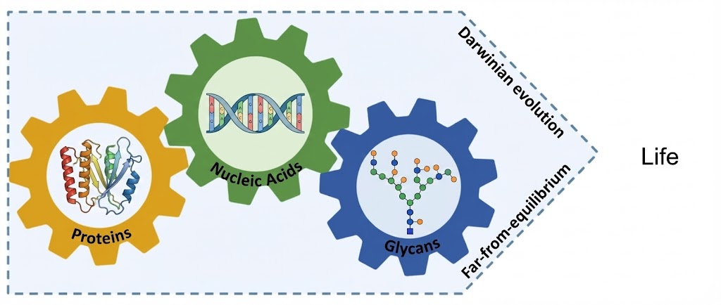
At the molecular level, life is composed of three biopolymers.

Glycans are made out of monosaccharides (e.g., glucose).
Proteins are made out of amino acids.
Nucleic acids are made out of nucleotides.

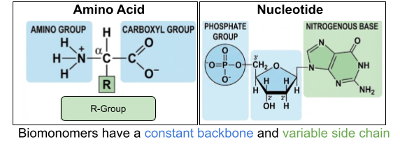
Most of our discussion will center on proteins and nucleic acids. Their constituents are themselves large, complex molecules. These monomers are built on an unchanging backbone and a variable side chain. For nucleotides, there are 4 available side chains (purine and pyrimidine nitrogenous bases). For amino acids, there are 20 available side chains (nonpolar, polar-uncharged, polar-positive, polar-negative R groups).

Organic polymers like polyesters aren’t particularly flexible. But biopolymers manifest extreme functional sophistication. And the polyfunctionality of nucleic acids and glycans must not be understated (Matange et al 2025).

Biopolymers also exhibit functional interdependence. Condensation of nucleotides is catalyzed by proteins, and condensation of amino acids is catalyzed by RNA. Biopolymers are heterocomplementary: proteins can recognize and bind to proteins, DNA, polyglycans, and small molecules. Nonbiological organic polymers do not manifest heterocomplementarity.

LUCA from Microbiology

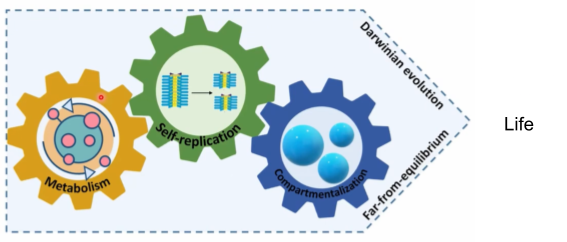
Another way to approach LUCA is to catalog biological universals: mechanisms shared by all life forms in existence. These universals can be organized in three categories: self-replication, metabolism, and compartmentalization. Let’s discuss each in turn.

The central genius of life was the discovery of proteins. By chaining amino acids together in long biopolymers, these polypeptides fold into arbitrary shapes. This invention is so powerful because in chemistry, structure determines function: arbitrary shapes unlock myriad potential behaviors. Proteins can form fibers, motors, containers, transporters, sensors, signals, optical devices, adhesives, pores, brushes, and pumps.

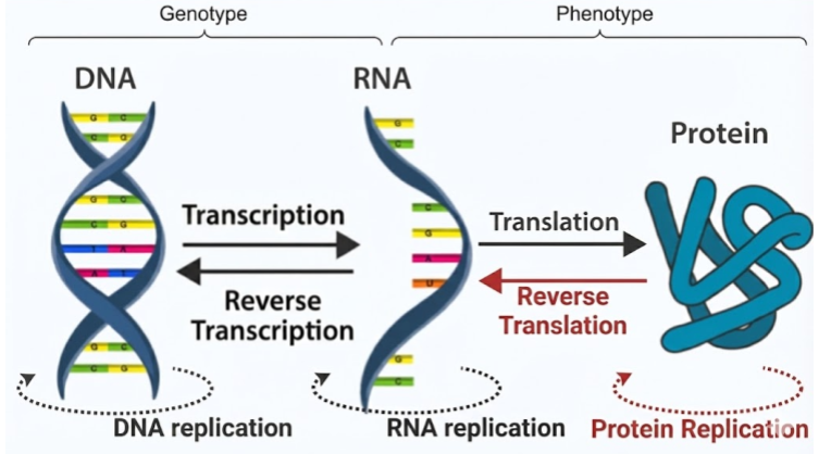
Proteins aren’t synthesized randomly – they are produced by template. Nucleotides combine together in long biopolymers known as nucleic acids. Double-stranded DNA is copied into single-stranded mRNA via the process of transcription. Then, during protein synthesis in the ribosome, codons (RNA triplets) specify which amino acids to attach in which order. This process of translation is defined by a codon-amino acid map known as the genetic code.

A gene is simply a patch of RNA that completely specifies a particular protein sequence. Your genome (genotype) is nothing more than a recipe for a proteome (phenotype). When philosophers speak of an innate desire to survive, that motivation must be carried by proteins. Natural selection operates on protein design. Nothing more and nothing less.

The Central Dogma describes the flow of information in biopolymers. The black arrows are allowed processes; the red arrows are not observed. Proteins cannot replicate because they are incapable of base pairing. Once information gets into a protein, it cannot get out again!

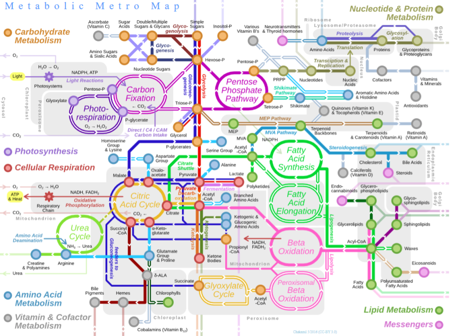
Why is life so fixated on proteins? To better understand this, it helps to consider metabolism. This is a chemical reaction network which provides two basic functions:

Catabolism (“energy metabolism”), a destructive process which breaks down complex compounds. This prominently includes pathways of cellular respiration, a controlled version of combustion in which glucose is slowly converted into carbon dioxide, water, and energy.
Anabolism (“carbon metabolism”), a constructive process which biosynthesizes new organic compounds. This includes pathways of carbon fixation (like Acetyl-CoA), which converts simple inorganic carbon dioxide into complex organics.

Enzymes are protein-based catalysts that reduce the activation energy of thermodynamically favorable (exergonic) reactions, speeding them up by many orders of magnitude. Some metabolic steps, however, are thermodynamically disfavorable (endergonic) and will not proceed spontaneously. Enzymes handle these by coupling them to a favorable reaction, making the combined process exergonic. The enzyme then catalyzes that coupled reaction in the usual way — by lowering its activation energy.

The 20 amino acids have a limited chemical repertoire; cofactors extend it — enabling electron transfer, redox chemistry, and group transfers that amino acid side chains cannot perform alone. There are two categories of cofactors: metal ions (e.g., Mg²⁺, and Fe²⁺), and organic molecules (i.e., coenzymes), many of which are derived from B vitamins (e.g., NAD). Without its cofactor, an enzyme (called an apoenzyme) is typically inactive. The complete, functional assembly is the holoenzyme.

Finally, while the Central Dogma traditionally depicts a linear flow of information from DNA to RNA to Protein, metabolism reveals that this dogma is actually a loop. Proteins are not just passive end-products; they are the active machinery required to synthesize and maintain the very DNA and RNA that encode them, creating a self-sustaining cycle of synthesis and regulation.

Modern metabolism and self-replication does not occur in an undifferentiated “primordial soup”. They occur inside impermeable membranes made of phospholipids.

Compartmentalization does a lot of heavy lifting at once: it shields nucleic acids from genetic parasites, buffers the system against environmental stress, and locally concentrates enzymes and substrates to speed reactions. By keeping metabolites and genetic material from simply diffusing away, it preserves hard-won products and information. Selective, protein-based gates regulate traffic—letting in foodstuffs, exporting waste—and can couple chemiosmosis to maintain a strong proton-motive force (≈3 pH units and ~200 mV), effectively a “cellular battery” that powers metabolic work. Finally, a stable compartment provides the physical unit that can reliably copy itself and propagate success via binary fission.

LUCA from Virology

Previous sections reconstructed LUCA as a cell. But modern oceans contain ten virions for every microbe. Viruses coevolve with cells, outnumber them, and may even predate them. Any reconstruction of early life that ignores them is incomplete.

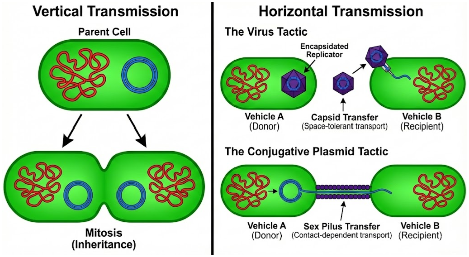
Once inside the cell, virulent viruses initiate the lytic cycle. Their genes hijack the host cell’s machinery to make more copies of themselves, ultimately rupturing the membrane and spilling newly-minted virions into the environment. They rely on horizontal transmission, in contrast to chromosomes which rely on vertical transmission via mitosis.

Viruses are not the only mobile genetic element (MGE) using horizontal transmission. Cells can contain small (often circular) nucleic acid outside of the chromosomes. These plasmids don’t kill the cell to transfer their DNA, but instead use conjugative sex pili to copy themselves into neighboring cells. Plasmid genetic material can be more similar to viruses than the chromosome. Some plasmids and viruses differ by no more than a capsid gene (Krupovic & Bamford 2010).

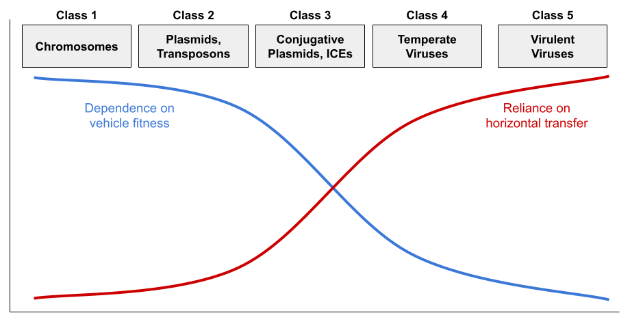
But virulence and conjugation are extremes. While virulent viruses are indifferent to cellular fitness, temperate viruses benefit from vertical transmission via the lysogenic cycle. They are thus less pathogenic. Some plasmids cannot construct the sex pilus and are capable of horizontal transmission only rarely. Jalasvuori (2012) shows that nucleic acids can be organized into a continuum:

This framework explains the distribution of replicator properties:

Class 3-5 all sense damage to the host cell, and initiate horizontal transfer when they detect vehicle stress. For example, herpesviruses reactivate from latency under host stress, producing cold sores.
Class 1 retains the core genome (e.g., DNA replication). Class 2-3 retain the accessory genome (e.g., virulence, antibiotic resistance).
Class 1-5 all retain addiction modules (a.k.a., MGE stabilization modules) like the toxin-antitoxin (TA) system (Mendoza-Guido & Rojas-Jimenez 2025). Many plasmids produce both a toxin and the antitoxin. Since the toxin has a longer half-life, loss of the plasmid entails death of the host. The restriction-modification (RM) system works in a very similar way (Kobayashi 2001).

There are three hypotheses for the origin of viruses:

The regression hypothesis claims that viruses are cells that progressively lost genetic information in their journey towards obligate parasitism.
The escape hypothesis claims that viruses originate from MGEs that gained increasingly sophisticated methods of horizontal transfer.
The virus-first hypothesis claims that viruses predate LUCA, originating from the primordial pool of replicators prior to the evolution of cells.

Dependent niches incentivize genome reduction. Mitochondria have transferred many genes to their host cells’ nuclei (Andersson & Kurland 1998), and parasitic bacteria like Rickettsia have shed much of theirs (Diop et al 2019). As obligate parasites, viruses should face the same reductive pressure — but what if they weren’t always parasitic? The discovery of giant viruses (in the phylum Nucleocytoviricota), with the first known translation-related machinery in a virus, was a revelation. In the spirit of the regression hypothesis, Boyer et al (2010) described them as living fossils of this fourth domain. But, while the relationship between reduction and parasitism is strong, recent phylogenetic work (Monttinen et al 2021) does not support this hypothesis.

The escape hypothesis accounts for some viral genes – particularly those encoding capsid proteins – which have clear cellular homologs. But viral hallmark genes, especially those involved in replication, are shared across diverse viral lineages yet absent from cellular genomes (Koonin et al 2006). If these genes escaped from cells, their cellular homologs should exist. Krupovic et al (2019) propose a chimeric origin that reconciles the escape and virus-first views. They argue that structural genes were captured from hosts, but replicator genes descend from primordial self-replicating elements that predate cells.

Theoretical models reinforce this view — selfish genetic elements arise inevitably in any replicator system, suggesting that genetic parasites have been components of life from the very beginning. Before replicators evolved error correction mechanisms, early replicators also faced a hard physical constraint known as Eigen’s error threshold: RNA replication error rates impose an upper bound on genome size. Viroids, the simplest known replicators at ~300 nucleotides, sit near this boundary. If the chimeric model is correct and viral replicator genes descend from primordial self-replicating elements, viroids may be the closest living relatives of those elements. Their structural simplicity, their lack of protein-coding capacity, and the recent discovery of viroid-like circular RNAs across diverse environments (Lee et al 2023) are all consistent with deep ancestry.

Looking Beyond the Root

The portrait above shows LUCA as anaerobic, prokaryotic, protein-dependent, chromosomally organized, besieged by viruses. But every feature of that portrait is also a choice made from a menu of alternatives that were never taken:

Alternative codes. Of ~500 amino acid species, only 20 are included in the genetic code, even though codons could distinguish up to 64. Central metabolites like ornithine, GABA, and β-alanine are biosynthesized but never translated.
Alternative replicator backbones. 5-carbon sugars (ribose, deoxyribose) are a strange choice for a nucleic acid backbone (Eschenmoser 1999). Chemists have built alternative replicators from 4-carbon sugars (TNA) and 3-carbon sugars (GNA).
Alternative protein backbones. Proteins are built from α-amino acids, but foldamers made from β, γ, and δ-amino acids can be more resistant to proteolysis and heat denaturation than their α-counterparts (Gellman 1998).

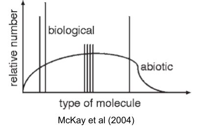
McKay (2004) captures this puzzle visually: nonbiological chemistry produces smooth distributions of organic molecules, but life uses only a sparse set of spikes against that background.

Each of these alternatives works better than what life uses, on some axis. So the interesting question isn’t whether LUCA could have been different; it’s why it wasn’t. Why haven’t we found shadow biospheres running on TNA, or β-peptide proteomes, or 34-amino-acid codes? Two possibilities: either we haven’t looked hard enough, or these choices were frozen so early and so deeply that no later lineage could back out of them. Both answers require understanding what happened before LUCA: the evolution of the ribosome, the freezing of the code, the crystallization of a chromosome out of competing replicators.

Beyond the root of the tree of life lies the origin. That’s the subject of our next post.

References

Andersson & Kurland (1998). Reductive evolution of resident genomes
Bowman et al (2020). Root of the Tree: The Significance, Evolution, and Origins of the Ribosome
Boyer et al (2010). Phylogenetic and Phyletic Studies of Informational Genes in Genomes Highlight Existence of a 4th Domain of Life Including Giant Viruses
Caforio, A., et al. (2018). “Converting Escherichia coli into an archaebacterium with a hybrid heterochiral membrane.”
Diop et al (2019). Paradoxical evolution of rickettsial genomes
Eschenmoser (1999). Chemical etiology of nucleic acid structure.
Forterre (2006). The origin of viruses and their possible roles in major evolutionary transitions.
Forterre et al (2013) Origin and Evolution of DNA and DNA Replication Machineries
Gellman (1998). Foldamers: A manifesto.
Harris et al (2003). The genetic core of the universal ancestor.
Jain et al (2014). Biosynthesis of archaeal membrane ether lipids
Jalasvuori (2012). Vehicles, replicators, and intercellular movement of genetic information: evolutionary dissection of a bacterial cell.
Koonin et al (2006). The ancient virus world and evolution of cells.
Kobayashi (2001). Behavior of restriction–modification systems as selfish mobile elements and their impact on genome evolution.
Krupovic et al (2019). Origin of viruses: primordial replicators recruiting capsids from hosts.
Krupovic & Bamford (2010). Order to the viral universe
Lee et al (2023). Mining metatranscriptomes reveals a vast world of viroid-like circular RNA
Matange et al (2025). Biological polymers: evolution, function, and significance.
McKay (2004). What Is Life—and How Do We Search for It in Other Worlds?
Mendoza-Guido & Rojas-Jimenez (2025). Beyond plasmid addiction: the role of toxin-antitoxin systems in the selfish behavior of mobile genetic elements.
Monttinen et al (2021). The genomes of nucleocytoplasmic large DNA viruses: viral evolution writ large

Fewer Lacunae

Distilled, Integrative Research

Tag science

The Reliability Ratio