OLS Estimation via Projection

Part Of: Machine Learning sequence
Content Summary: 800 words, 8 min read

Projection as Geometric Approximation

If we have a vector $b$ and a line determined by vector $a$ , how do we find the point on the line that is closest to $b$ ?

OLS- Geometry of Projection

The closest point $p$ is at the intersection formed by a line through $b$ that is orthogonal to $a$ . If we think of $p$ as an approximation to $b$ , then the length of $e = b - p$ is the error of that approximation.

$a^T e = a^T (b - ax) = 0$

This formula captures projection onto a vector. But what if you want to project to a higher dimensional surface?

Imagine a plane, whose basis vectors are $a_1$ and $a_2$ . This plane can be described with a matrix, by mapping the basis vectors onto its column space:

$A = \begin{bmatrix} a_1 & a_2 \end{bmatrix}$

Suppose we want to project vector $b$ onto this plane. We can use the same orthogonality principle as before:

$A^Te = A^T(b-Ax) = 0$

$A^TAx = A^Tb$

Matrices like $A^TA$ are self-transpositions. We have shown that such matrices are square symmetric, and thereby contain positive, real eigenvalues.

We shall assume that the columns of $A^TA$ are independent, and it thereby is invertible. The inverse thereby allows us to solve for $x$ :

$(A^TA)^{-1}(A^TA)x = (A^TA)^{-1}A^Tb$

$x = (A^TA)^{-1}A^Tb$

Recall that,

$p = Ax = A(A^TA)^{-1}A^Tb$

Since matrices are linear transformations (functions that operate on vectors), it is natural to express the problem in terms of a projection matrix $P$ , that accepts a vector $b$ , and outputs the approximating vector $p$ :

$p = Pb$

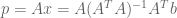
By combining these two formula, we solve for $P$ :

$P = A(A^TA)^{-1}A^T$

Thus, we have two perspectives on the same underlying formula:

OLS- Regression Functions via Matrices (1)

Linear Regression via Projection

We have previously noted that machine learning attempts to approximate the shape of the data. Prediction functions include classification (discrete output) and regression (continuous output).

Consider an example with three data points. Can we predict the price of the next item, given its size?

OLS- Regression Function Setup

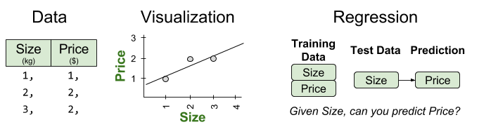
For these data, a linear regression function will take the following form:

$\psi : Size \rightarrow Price$

$\psi(Size) = \beta_0 + \beta_1 Size$

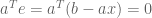
We can thus interpret linear regression as an attempt to solve $Ax=b$ :

OLS- Linear Algebra Regression Matrix

In this example, we have more data than parameters (3 vs 2). In real-world problems, it is an extremely common predicament. It yields matrices with may more equations than unknowns. This means that $Ax=b$ has no solution (unless all data happen to fall on a straight line).

If exact solutions are impossible, we can still hope for an approximating solution. Perhaps we can find a vector p that best approximates b. More formally, we desire some $p = A\bar{x}$ such that the error $e = b-p$ is minimized.

Since projection is a form of approximation, we can use a projection matrix to construct our linear prediction function $\psi : Size \rightarrow Price$ .

OLS- Least Squares Fundamental Spaces

A Worked Example

The solution is to make the error $b-Ax$ as small as possible. Since $Ax$ can never leave the column space, choose the closest point to $b$ in that subspace. This point is the projection $p$ . Then the error vector $e = b-p$ has minimal length.

To repeat, the best combination $p = Ax$ is the projection of b onto the column space. The error is perpendicular to that subspace. Therefore $e = b-p$ is in the left nullspace:

$Ax = b$

$A^TA = \begin{bmatrix} 1 & 1 & 1 \\ 1 & 2 & 3 \\ \end{bmatrix} \begin{bmatrix} 1 & 1 \\ 1 & 2 \\ 1 & 3 \\ \end{bmatrix} = \begin{bmatrix} 3 & 6 \\ 6 & 14 \\ \end{bmatrix}$

We can use Guass-Jordan Elimination to compute the inversion:

$(A^TA)^{-1} = \begin{bmatrix} 7/3 & -1 \\ -1 & 1/2 \\ \end{bmatrix}$

A useful intermediate quantity is as follows:

$(A^TA)^{-1}A^T = \begin{bmatrix} 7/3 & -1 \\ -1 & 1/2 \\ \end{bmatrix} \begin{bmatrix} 1 & 1 & 1 \\ 1 & 2 & 3 \\ \end{bmatrix} = \begin{bmatrix} 4/3 & 1/3 & -2/3 \\ -1/2 & 0 & 1/2 \\ \end{bmatrix}$

We are now able to compute the parameters of our model, $\bar{x}$ :

$\bar{x} = \left[ (A^TA)^{-1}A^T \right] b = \begin{bmatrix} 4/3 & 1/3 & -2/3 \\ -1/2 & 0 & 1/2 \\ \end{bmatrix} \begin{bmatrix} 1 \\ 2 \\ 2 \\ \end{bmatrix} = \begin{bmatrix} 2/3 \\ 1/2 \\ \end{bmatrix}$

These parameters generate a predictive function with the following structure:

$\psi : Size \rightarrow Price$

$\psi(Size) = \frac{2}{3} + \frac{1}{2}Size$

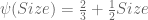
These values correspond with the line that best fits our original data!

Wrapping Up

Takeaways:

In linear algebra, projection approximates a high-dimensional surface in a lower-dimensional space. The projection error can be measured.
In linear regression, we usually cannot solve $Ax=b$ , because there tends to be more data than parameters ( $b$ is not in the column space)
We can find the closest vector in the column space by projecting onto $b$ , and minimizing the projection error.
Thus, the operation of projection can be used to perform parameter estimation, and produce a model that best approximates the training data.

Related Resources:

This article is largely based on MIT lecture Projections onto Subspaces and Projection Matrices and Least Squares. If you’d like to test whether you understood this method, try the example problems for yourself!

Fewer Lacunae

Distilled, Integrative Research

OLS Estimation via Projection

Leave a Reply Cancel reply

Share this:

Like this:

Related

Leave a Reply Cancel reply