Part Of: Machine Learning sequence
Followup To: OLS Estimation via Projection
Content Summary: 4800 words, 24 min read

The Reliability Ratio

A student scores 2 standard deviations (SD) above the mean on an exam, in about the top 2%. A month later she retakes the exam. Even if nothing about her changes, her second exam score will probably be lower. How much lower? One number answers this question: the reliability ($λ$) of the test.

To understand reliability, classical test theory (CTT) splits her score into two steps. Write it as $x = s + n$. The first step, the signal s, runs from the population mean to the student’s true score: the average she would earn over many sittings. The second step, the noise n, runs from her true score to her observed score.

Let’s imagine each true score is a type. Students of the same type still get different scores, because each sitting draws its own error. Suppose type k has true score $s_k$ and makes up a fraction $p_k$ of the population. Each distribution of types is the normal distribution $\mathcal{N}\big(s_k, \operatorname{Var}(n)\big)$. The population is their weighted sum:

$f(x) = \sum_k p_k , \mathcal{N}\big(s_k, \operatorname{Var}(n)\big)$

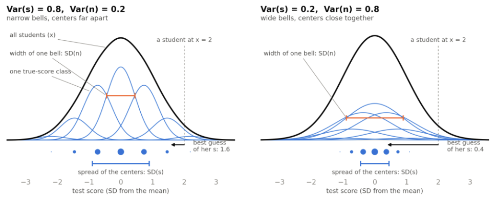
The same distribution of observed scores can come from two different situations. One sitting per student cannot tell the two situations apart.

Because n is independent of s, the two variances add:

$\operatorname{Var}(x) = \operatorname{Var}(s) + \operatorname{Var}(n)$

To see why, square a student’s deviation: $(s+n)^2 = s^2 + 2sn + n^2$. Average each term over all students. The first gives $Var(s)$, and the last gives $Var(n)$. Inside one bell, s is fixed and n averages to zero, so the cross term $2sn$ also averages to zero.

Because the variances add, each one is a share of the whole. The share that comes from true scores is the reliability of the test:

$\text{Reliability: } \lambda = \frac{\operatorname{Var}(s)}{\operatorname{Var}(x)}$

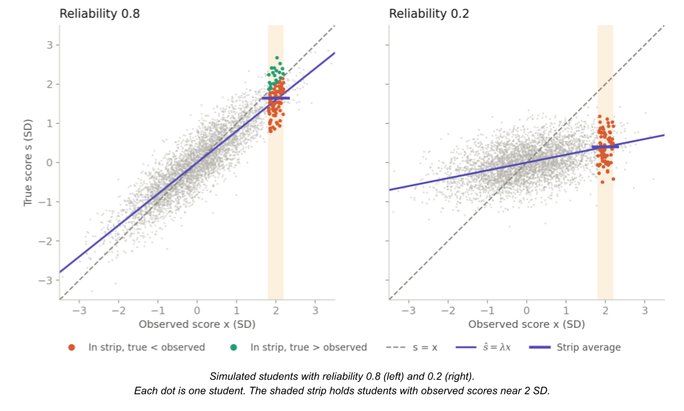
It runs from 0 to 1, and the error share is 1 − λ. In the figure, Var(x) = 1, so λ is 0.8 on the left and 0.2 on the right. So λ describes a test in one population. Give the same test to a narrower population, and Var(s) falls while Var(n) stays the same, so λ falls.

The Coefficient of Determination

Reliability answers a question: how much of the variance in observed scores does the true score predict? Regression answers the same question with the coefficient of determination.

Regress an outcome y on one predictor. The fitted line makes a prediction ŷᵢ for each observation, and the residual $eᵢ = yᵢ − ŷᵢ$ is the error that remains.

A model’s mean squared error (MSE) measures the performance of the model:

$\text{MSE}{\text{model}} = \frac{1}{N}\sum_i (y_i – \hat{y}i)^2 = \frac{1}{N}\sum_i e_i^2$

The coefficient of determination (R²) measures how well the model’s predictions track the outcome. It compares the model’s MSE with a baseline that predicts the mean ȳ for every observation:

$\text{MSE}{\text{base}} = \frac{1}{N}\sum_i (y_i – \bar y)^2 = \operatorname{Var}(y) R^2 = 1 – \frac{\text{MSE}{\text{model}}}{\text{MSE}{\text{base}}}$

If the model predicts every observation exactly, R² = 1. If it matches the baseline, R² = 0.

Two properties of least squares will be used in this section. First, the residuals average to zero. Second, they are uncorrelated with the predictions.

Given the first property, and the fact that a variable with zero mean has a variance equal to its mean square:

$\text{MSE}{\text{model}} = \frac{1}{N}\sum_i e_i^2 = \operatorname{Var}(e).$

We can now write the coefficient of determination in terms of variances:

$R^2 = 1 – \frac{\operatorname{Var}(e)}{\operatorname{Var}(y)} = \frac{\operatorname{Var}(y) – \operatorname{Var}(e)}{\operatorname{Var}(y)}$

The second property splits the variance of the outcome. Since y = ŷ + e, its variance is,

$\operatorname{Var}(\hat y + e) = \operatorname{Var}(\hat y) + \operatorname{Var}(e) + 2\operatorname{Cov}(\hat y, e)$

The covariance term is zero, so

$\operatorname{Var}(y) = \operatorname{Var}(\hat y) + \operatorname{Var}(e)$

Substitute this into the numerator:

$R^2 = \frac{\operatorname{Var}(\hat y)}{\operatorname{Var}(y)}$

This equation is why R² is also called the explained variance.

In CTT, the noise n has both properties, so x = s + n is a least-squares regression with fit x̂ = s. We cannot run this regression, because true scores are hidden. Its R² still exists, and it is the reliability:

$R^2 = \frac{\operatorname{Var}(\hat x)}{\operatorname{Var}(x)} = \frac{\operatorname{Var}(s)}{\operatorname{Var}(x)} = \lambda$

CTT assumes these properties. In regression, least squares provides them for the training data. On new data, the model can underperform baseline, and R² can be negative.

The Geometry of Variance

OLS Estimation via Projection showed that least squares projects a vector onto the column space of a matrix A. The residual e is perpendicular to that space: $A^\top e = 0$. The same geometry organizes variance.

Treat each variable as a vector with one entry for each of the N students. Subtract the mean from each entry, and divide each entry by √N. The covariance is an average of products:

$\operatorname{Cov}(u, v) = \frac{1}{N}\sum_{i=1}^{N} (u_i – \bar u)(v_i – \bar v)$

Each vector carries a factor of 1/√N, so their dot product carries 1/N. For these vectors, statistics and geometry are related by the following identities.

$\operatorname{Cov}(u, v) = u \cdot v, \qquad \operatorname{Var}(u) = |u|^2, \qquad \sigma_u = |u|$

The correlation (r) of two variables is the covariance of their standardized versions, $z_u = u/\sigma_u$ and $z_v = v/\sigma_v$. In vector terms, this divides the dot product by both lengths, which gives the cosine of the angle between the vectors:

$\text{Correlation: } r = \frac{\operatorname{Cov}(u, v)}{\sigma_u \sigma_v} = \operatorname{Cov}(z_u, z_v) = \frac{u \cdot v}{|u|,|v|} = \cos\theta$

Two uncorrelated variables have r = 0 = cos 90°, so they are perpendicular.

Signal and noise are uncorrelated, so they are perpendicular, and $x = s + n$ is the hypotenuse of a right triangle. The legs have lengths $\sigma_s = 4$ and $\sigma_n = 3$, and the hypotenuse has length $\sigma_x = 5$. The lengths do not add: 4 + 3 ≠ 5. The areas of the squares on the sides are the variances, and they do add: 16 + 9 = 25. In this geometry, variance additivity is the Pythagorean theorem. Fisher (1918) introduced the term variance because of this additivity.

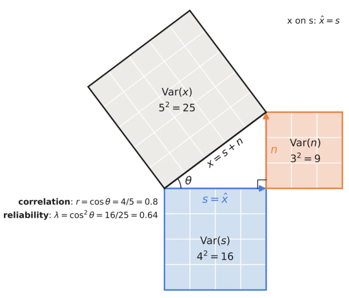
The split $Var(y) = Var(ŷ) + Var(e)$ in the previous section is the same theorem. The prediction and the residual are uncorrelated, so they are perpendicular. Because the vectors are centered, a regression on one predictor projects the outcome onto the predictor.

For an outcome v and a predictor u, the residual $v − bu$ is perpendicular to u, so $u · (v − bu) = 0$. Write $b_{v|u}$ for the slope of v on u.

$b_{v|u} = \frac{u \cdot v}{u \cdot u} = \frac{\operatorname{Cov}(u, v)}{\operatorname{Var}(u)}$

The slope is the covariance of the predictor and the outcome, divided by the variance of the predictor. The triangle shows the regression of x on s from the previous section. The residual n is perpendicular to the predictor s, so the fit is s itself, and b_{x|s} = 1.

The side s is adjacent to the angle θ, and x is the hypotenuse, so

$r = \cos\theta = \frac{|s|}{|x|} = \frac{\sigma_s}{\sigma_x} = \frac{4}{5} = 0.8$

$\lambda = R^2 = \frac{|s|^2}{|x|^2} = \cos^2\theta = r^2 = \frac{16}{25} = 0.64$

The reliability is the squared correlation between true and observed scores. This holds for any regression with one predictor:

$R^2 = \cos^2\theta = r^2$

Regression to the Mean

The slope of y on x is $Cov(x, y)/Var(x)$. Measure both variables in standard deviations, and the slope becomes r. The slope of x on y is also r. In any units, the two slopes multiply to r²:

$b_{y|x}, b_{x|y} = \frac{\operatorname{Cov}(x,y)}{\operatorname{Var}(x)} \cdot \frac{\operatorname{Cov}(x,y)}{\operatorname{Var}(y)} = r^2$

In standard units, unless the correlation is exact, every prediction is less extreme than its predictor. Galton (1886) found this in human stature. He compared the heights of children with the mean height of their parents and found a slope of about two thirds: parents whose mean height is 3 inches above average have children about 2 inches above average. He called this effect regression towards mediocrity. We now call it regression to the mean.

The slope of about two thirds is measured in inches per inch. It differs from the correlation because parental averages vary less than children’s heights.

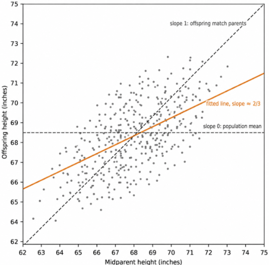
Regression to the mean also runs backward in time: tall children have parents who are, on average, less tall than they are. The effect doesn’t require a causal mechanism. It manifests whenever measurements share a signal but also draw independent noise.

When a test is administered twice, for example, the two sittings share a true score and nothing else, so their covariance is Var(s). They also have the same variance, Var(x). So the slope of retest on test and their correlation are both $Var(s)/Var(x) = λ$.

Galton’s data has the same structure. The mid-parent height is a noisy measure of the parents’ mean additive genetic value: the part of genetic value that children inherit on average. A child inherits that value and draws new noise of its own. So the covariance of child and mid-parent is the variance of the genetic signal, and the slope of child on mid-parent is a reliability ratio. The child’s height varies more than the mid-parent’s, so here only the slope equals this ratio. Quantitative genetics calls this ratio heritability. Under simple genetic assumptions, Galton’s slope of about two thirds measures the heritability of height.

Reliability is the slope of retest on test. It is the component of a result that carries over to the next measurement.

Shrinkage

Recall our student with a strong test score. Regression to the mean says her retest will probably be lower. What is her true score?
The geometry section knew the true score (s) and predicted the observed score (x). It regressed x on s. Our student’s case runs the other way. We know only her observed score, so we regress s on x to estimate her true score.

Independent noise adds nothing to a covariance, so the covariance of the true and observed scores is the variance of the signal:
$\operatorname{Cov}(s, x) = \operatorname{Var}(s)$

A slope is this covariance divided by the variance of the predictor, so only the denominator changes:

$b_{x|s} = \frac{\operatorname{Var}(s)}{\operatorname{Var}(s)} = 1, \qquad b_{s|x} = \frac{\operatorname{Var}(s)}{\operatorname{Var}(x)} = \lambda$

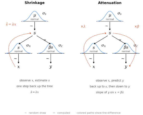
If we know a student’s true score, her observed score averages to that true score. When true scores and errors are normal, no curve does better than the line ŝ = λx. This estimate is called Kelley’s rule. Kelley (1927) derived it in the context of test scores. It is a weighted average of the test score X and the population mean μ:

$\hat{s}_{\text{raw}} = \lambda X + (1-\lambda)\mu$

If the test has high reliability, the estimator trusts the score. Else, it trusts the population mean.

Consider students who achieve a test score of 2 SD. By definition of the normal distribution, many of these students have a true score near 1 SD. So an observed score of 2 SD comes more often from a good student with good luck than from an excellent student with average luck. Consider one of these students. Reliability tells us how much of her lead is skill. With a reliability of 0.8, about 80% of her 2 SD lead is skill, so her best-guess true score is about 1.6 SD.

A Kalman filter (Kalman 1960) tracks a hidden quantity with a current estimate. The estimate’s error has variance P, and each measurement adds noise with variance R. These play the same roles of Var(s) and Var(n) in CTT. The estimate has variance P + R. The filter moves its estimate toward the measurement by a weight K called the gain:

$K = \frac{\operatorname{Var}(\text{true step})}{\operatorname{Var}(\text{measured step})} = \frac{P}{P + R}$

The Kalman filter uses Kelley’s rule, but with the current estimate in place of the population mean. A noisy measurement has a small gain and is largely ignored.

Reliability is also a shrinkage factor. It is the share of an observed lead that we credit to the true score.

Attenuated Slopes

The true scores are often latent, but estimating them can enable downstream predictions. An epidemiologist wants to know how much stroke risk rises with blood pressure. She needs the slope of stroke risk y on each patient’s usual blood pressure s. But she has only one reading x per patient, a noisy measure of s. If she regresses stroke risk on the readings, what slope does she get?

Suppose an outcome depends on the true score, $y = βs + ε$. The slope we want is $b_{y|s} = \beta$. True scores are hidden, so we can fit only $b_{y|x}$, the regression of y on the observed score x = s + n. Write $\lambda_x$ for the reliability of x.

$x = s + n,\quad y = \beta s + \varepsilon,\quad b_{y|x} = \frac{\operatorname{Cov}(y,\ x)}{\operatorname{Var}(x)} = \frac{\operatorname{Cov}(\beta s + \varepsilon,\ s + n)}{\operatorname{Var}(x)}$

If we assume the noise n and the error ε are independent of s and of each other, they add nothing to the covariance:

$\operatorname{Cov}(\beta s + \varepsilon,\ s + n) = \beta\operatorname{Var}(s) + \beta\operatorname{Cov}(s, n) + \operatorname{Cov}(\varepsilon, s) + \operatorname{Cov}(\varepsilon, n) = \beta\operatorname{Var}(s)$

$b_{y|x} = \frac{\operatorname{Cov}(\beta s + \varepsilon,\ s + n)}{\operatorname{Var}(x)} = \beta,\frac{\operatorname{Var}(s)}{\operatorname{Var}(x)} = b_{y|s}, b_{s|x} = \beta\lambda_x$

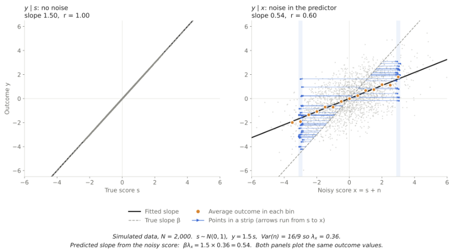
The slope from a noisy predictor is a product of two factors. The first shrinks the observed score to estimated true score by the reliability. The second factor β carries the true score to the outcome. This process is known as attenuation bias, or regression dilution.

An illustration of the shrinkage. Adding noise to the predictor is visualized as horizontal arrows. The slope of the estimated function flattens.

Her slope from the readings is $\beta\lambda_x$. For predicting stroke from one reading, this is the best slope she can use. To recover β itself, she divides her slope by $\lambda_x$, which she can estimate from repeated readings on some of her patients. MacMahon et al. (1990) made this correction in studies of blood pressure and heart disease. The corrected associations with stroke and coronary heart disease were about 60% stronger than the uncorrected ones.

A related effect appears in models trained on many features. Suppose the model also sees a feature z that correlates with the true score s. Then z takes over part of the weight that x loses, even if z has no effect on the outcome. If s is a confounder, epidemiologists call the bias that remains after adjusting for x residual confounding (Phillips & Davey Smith 1991).

Attenuated Correlations

Suppose we score a model against labels from one radiologist. The labels are a noisy measure of the true outcome. Write the radiologist’s label as

$\tilde{y} = y + \delta$

where δ is the radiologist’s error, independent of s, n, and ε. How does label noise change the slope and the correlation?

In the algebra, δ adds nothing to the covariance, so the slope is unchanged:

$b_{\tilde y|x} = \frac{\operatorname{Cov}(y + \delta,\ x)}{\operatorname{Var}(x)} = \frac{\operatorname{Cov}(y,\ x)}{\operatorname{Var}(x)} = b_{y|x}$

But the noisy label does attenuate the correlation. Recall our definitions.

$r_{\text{true}} = \frac{\operatorname{Cov}(s,\ y)}{\sigma_s,\sigma_y}, \qquad r_{\text{observed}} = \frac{\operatorname{Cov}(x,\ \tilde y)}{\sigma_x,\sigma_{\tilde y}}$

The noises are independent, so the numerators are equal.

$\operatorname{Cov}(x,\ \tilde y) = \operatorname{Cov}(s + n,\ y + \delta) = \operatorname{Cov}(s,\ y)$

Multiply the true correlation by a ratio of standard deviations to get the observed correlation:

Both reliability ratios reduce the correlation, so observed correlations are closer to zero than true correlations.

Spearman (1904) named this weakening attenuation. To correct an observed correlation, divide it by$(\lambda_x \lambda_y)^{1/2}$.

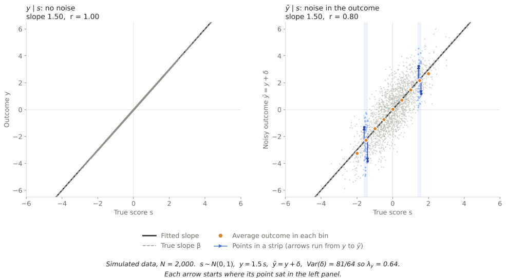
In the figure, the left panel has no noise. In the right panel, each point moves up or down by its noise, and its true score stays the same. The noise averages to zero in each bin, so the orange dots stay on the true line, and the slope stays at 1.5. The correlation falls from 1 to ${\lambda_y}^{1/2} = 0.8$.

These are the regressions of this post, each with its slope and correlation.

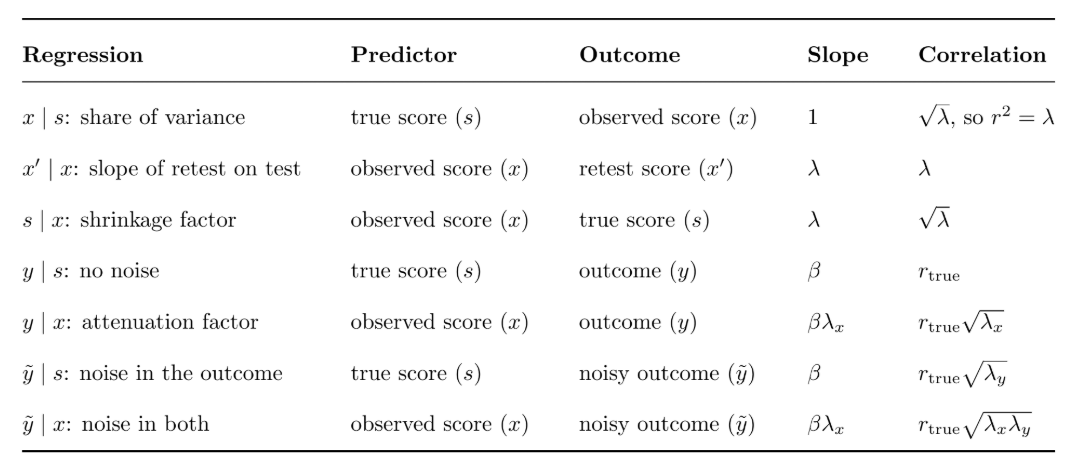
Reliability is also an attenuation factor. A noisy predictor keeps the share λ of a true slope, and each noisy measurement keeps the share √λ of a true correlation.

Estimating Reliability

So far, we have treated the reliability λ as known. In practice, we must estimate it. One score per student cannot provide an estimate, but a second score of the same student can. Since test and retest share the true score and nothing else, we saw that their correlation was λ. More sittings give a better estimate of λ, and their average is a more reliable score.

Suppose each of N students sits the test m times. The score of student i on sitting j, and her average across all sittings are:

$x_{ij} = s_i + n_{ij}, \qquad \bar{x}_i = s_i + \bar{n}_i$

The true score and the errors are independent, so their variances add

$\operatorname{Var}(\bar{x}_i) = \operatorname{Var}(s) + \operatorname{Var}(\bar{n}_i) = \operatorname{Var}(s) + \frac{\operatorname{Var}(n)}{m}$

Across m sittings, the reliability of the average $\lambda_m$ is the share of this variance that comes from the true score.

$\lambda_m = \frac{\operatorname{Var}(s)}{\operatorname{Var}(\bar{x}_i)} = \frac{\operatorname{Var}(s)}{\operatorname{Var}(s) + \operatorname{Var}(n)/m}$

For one sitting, recall the signal share and error share:

$\lambda = \frac{\operatorname{Var}(s)}{\operatorname{Var}(x)} \qquad 1-\lambda = \frac{\operatorname{Var}(n)}{\operatorname{Var}(x)}$

The relationship between reliability of the average and single-sitting reliability is known as the Spearman-Brown formula (Spearman 1910; Brown 1910).

$\lambda_m = \frac{m\lambda}{1 + (m-1)\lambda}$

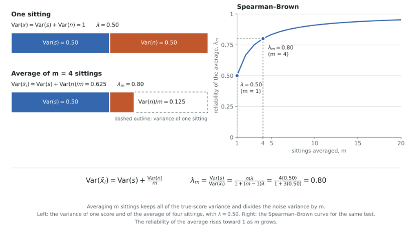
Repeated sittings also let us estimate the signal and noise variances. The spread of each student’s scores around her own average estimates Var(n). The spread of the student averages around the grand average x̄, the average of all the scores, estimates Var(x̄ᵢ):

$\widehat{\operatorname{Var}}(n) = \frac{1}{N(m-1)}\sum_{i=1}^{N}\sum_{j=1}^{m}\left(x_{ij}-\bar{x}_i\right)^2 \qquad \widehat{\operatorname{Var}}(\bar{x}i) = \frac{1}{N-1}\sum{i=1}^{N}\left(\bar{x}_i-\bar{x}\right)^2$

These divisors differ from the 1/N of earlier sections. Scores sit closer to their own average than to their true mean, so dividing by the number of scores would give too small an estimate. Each divisor counts degrees of freedom: m – 1 inside each of the N students, and N – 1 for the averages.

Replace each variance in the equation for the variance of the average with its estimate, solve for the signal variance, and substitute the estimates into both reliabilities:

$\widehat{\operatorname{Var}}(s) = \widehat{\operatorname{Var}}(\bar{x}_i) – \frac{\widehat{\operatorname{Var}}(n)}{m} \qquad \hat{\lambda} = \frac{\widehat{\operatorname{Var}}(s)}{\widehat{\operatorname{Var}}(s) + \widehat{\operatorname{Var}}(n)} \qquad \hat{\lambda}_m = \frac{\widehat{\operatorname{Var}}(s)}{\widehat{\operatorname{Var}}(s) + \widehat{\operatorname{Var}}(n)/m}$

Thus, the Spearman–Brown formula can be applied to estimate λ and $\lambda_m$.

This method is the analysis of variance (ANOVA), and Hoyt (1941) used it to estimate reliability. ANOVA states both spreads on the scale of one sitting, as the mean square within (MSW) and the mean square between (MSB).

$\text{MSW} = \widehat{\operatorname{Var}}(n) \qquad \text{MSB} = m,\widehat{\operatorname{Var}}(\bar{x}_i)$

More sittings make the noise estimate precise. Only more students make the signal estimate precise, because the spread of the averages has N-1 degrees of freedom.

A retest needs a second sitting. Cronbach’s alpha (Cronbach 1951) estimates reliability from one sitting. Each question acts as a short retest of the same true score. So each covariance between two questions estimates the signal variance, and each question’s variance estimates the variance of one score. The average covariance c over the average variance v then estimates the reliability of one question. This estimate assumes that every question measures the true score equally strongly. The m questions play the role of m sittings, and the total score has the same reliability as their average. So the Spearman–Brown formula gives alpha:

$\alpha = \frac{m,c/v}{1 + (m-1),c/v} = \frac{m,c}{v + (m-1),c}$

Psychometricians use alpha to build tests: they keep the questions that raise alpha and drop the ones that lower it.

The two formulas average over different replications. For reliability of the average, the replications are m sittings of the same test on different days. For alpha, they are the m questions of one sitting. Retest reliability and Cronbach’s alpha can differ for the same test. A more granular analysis of variance explains the divergence. Divide each score into four parts:

• Ability (e.g., intelligence)
• Day state (e.g., sleep or mood)
• Question fit (e.g., having studied these topics)
• Leftover (e.g., a lucky guess)

Administering a test again on a different day keeps only ability and question fit. Administering different questions in one sitting retains ability and day state. This approach to variance is further elaborated in generalizability theory (Cronbach et al. 1972).

Hierarchical Models

CTT has two levels: students taking multiple tests (i.e., sittings). A hierarchical model (HM) has two levels, but at a different granularity: groups having multiple members. In HM, each score is an observation of the group mean. Sittings are glossed over as part of the individual variance.

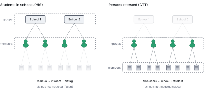
Many of our CTT constructs reappear in HM with new labels.

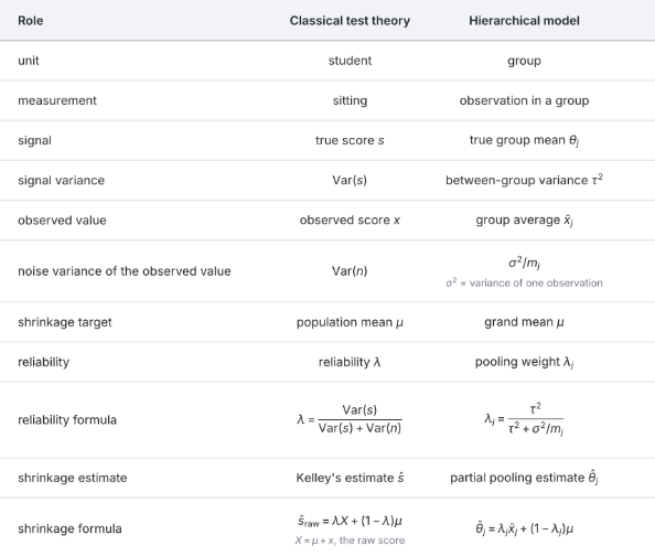
CTT gives every student the same number of sittings, but HM lets groups differ in size. Let mⱼ be the number of students in school j. A school with 20 students and a school with 2,000 students might each report average test scores, and the score of the former is much noisier. Let τ² denote the variance of the true group scores, and σ² denote the variance of student scores within the school. The Spearman–Brown formula gives the reliability of each school:

$\lambda_j = \frac{\tau^2}{\tau^2 + \sigma^2/m_j}$

The estimate of each group mean is Kelley’s rule, with the grand mean μ in place of the population mean:

$\hat{\theta}_j = \lambda_j,\bar{x}_j + (1-\lambda_j),\mu$

Statisticians call this estimate partial pooling. It is a compromise between no pooling (each school keeps its own score) and complete pooling (every group is estimated with the grand mean). Each estimate θ̂ⱼ depends on τ², σ², and μ, and all three come from every group. So each estimate uses information from the other groups. This is known as borrowing strength.

With equal sizes, one weight scales every average, and the rank order stays the same. With unequal sizes, small groups move further toward the grand mean than large groups, so groups can change rank. Wainer (2007) described a case from education. Small schools were overrepresented among the schools with the highest test scores, and this result encouraged large investments in smaller schools. Small schools were also overrepresented among the schools with the lowest scores.

Wainer named the rule behind this pattern de Moivre’s equation: the error of an average of m observations has standard deviation σ/√m. A small school averages few students, so its average has a large error. Large errors put small schools in both tails. The same rule puts small units in both tails in other domains. The US counties with the highest and the lowest kidney cancer death rates are mostly small rural counties (Gelman & Price 1999). Hospitals that treat few patients have the most extreme death rates (Spiegelhalter 2005). Products with few reviews fill both ends of rating lists. Partial pooling moves these small units toward the grand mean.

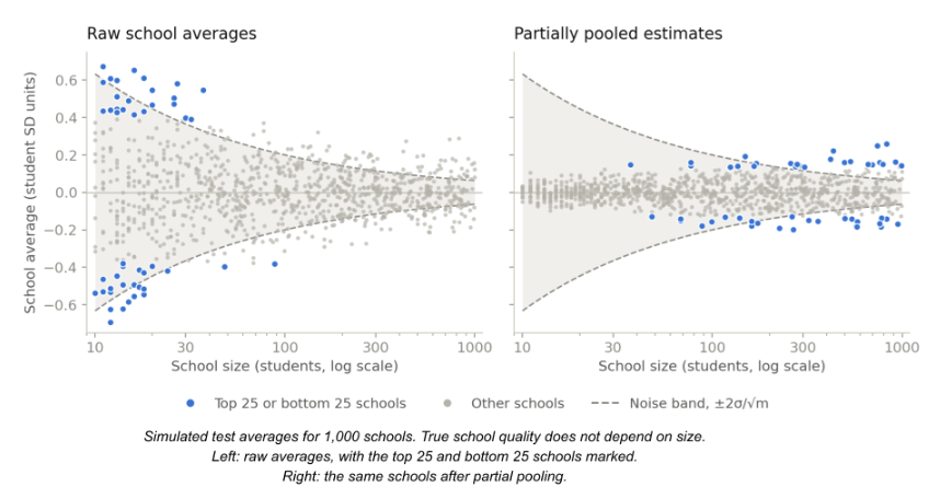
In the left panel, all 50 of the most extreme schools have fewer than 100 students. In the right panel, the extremes are now mostly large schools.

Reliability is also a pooling weight. It is the share of its own average that each group keeps.

Reliability and Regularization

Intro to Regularization added a penalty on the size of a model’s weights. With standardized and uncorrelated features, this ridge penalty shrinks each least-squares weight toward zero by a factor with the same form as the reliability ratio (Hastie et al. 2009). An unregularized fit corresponds to perfect reliability, taking the data at face value. Training on inputs with added noise has the same effect as ridge regression for linear models (Bishop 1995), so attenuation is also a form of regularization.

Maximum likelihood estimation (MLE) estimates each mean by its observed value. But noise accumulates, and the estimate vector is too long on average. Stein (1956) showed that for three or more means, the MLE is inadmissible: another estimator has lower expected total squared error for every possible set of true means. The means can be unrelated, which is why the result is called Stein’s paradox. James & Stein (1961) gave such an estimator. It pulls every estimate toward zero by one shared reliability factor: the share of the estimates’ squared size that comes from the true means.

Model selection compares candidate models and keeps the one with the best score. Any score used to make this choice is optimistic. The winner probably had good luck on the scoring data, and its score will probably decrease on fresh data. This phenomenon of selection bias (Cawley & Talbot 2010) is another form of regression to the mean. Bidders in auctions call it the winner’s curse (Capen et al. 1971). Data partitioning creates a retest. An untouched holdout set draws fresh luck, so its score is honest.

Wrapping Up

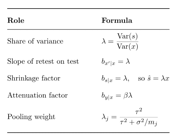
The reliability λ plays five roles:

References

• Bishop (1995). Training with noise is equivalent to Tikhonov regularization.
• Brown (1910). Some experimental results in the correlation of mental abilities.
• Capen, Clapp & Campbell (1971). Competitive bidding in high-risk situations.
• Cawley & Talbot (2010). On over-fitting in model selection and subsequent selection bias in performance evaluation.
• Cronbach (1951). Coefficient alpha and the internal structure of tests.
• Cronbach et al. (1972). The Dependability of Behavioral Measurements.
• Fisher (1918). The correlation between relatives on the supposition of Mendelian inheritance.
• Galton (1886). Regression towards mediocrity in hereditary stature.
• Gelman & Price (1999). All maps of parameter estimates are misleading.
• Hastie, Tibshirani & Friedman (2009). The Elements of Statistical Learning.
• Hoyt (1941). Test reliability estimated by analysis of variance.
• James & Stein (1961). Estimation with quadratic loss.
• Kalman (1960). A new approach to linear filtering and prediction problems.
• Kelley (1927). Interpretation of Educational Measurements.
• MacMahon et al. (1990). Blood pressure, stroke, and coronary heart disease. Part 1, prolonged differences in blood pressure: prospective observational studies corrected for the regression dilution bias.
• Phillips & Davey Smith (1991). How independent are “independent” effects? Relative risk estimation when correlated exposures are measured imprecisely.
• Spearman (1904). The proof and measurement of association between two things.
• Spearman (1910). Correlation calculated from faulty data.
• Spiegelhalter (2005). Funnel plots for comparing institutional performance.
• Stein (1956). Inadmissibility of the usual estimator for the mean of a multivariate normal distribution.
• Wainer (2007). The most dangerous equation.