The Reliability Ratio

Part Of: Machine Learning sequence
Followup To: OLS Estimation via Projection
Content Summary: 4800 words, 24 min read

The Reliability Ratio

A student scores 2 standard deviations (SD) above the mean on an exam, in about the top 2%. A month later she retakes the exam. Even if nothing about her changes, her second exam score will probably be lower. How much lower? One number answers this question: the reliability (λλ) of the test.

To understand reliability, classical test theory (CTT) splits her score into two steps. Write it as x=s+nx = s + n. The first step, the signal s, runs from the population mean to the student’s true score: the average she would earn over many sittings. The second step, the noise n, runs from her true score to her observed score.

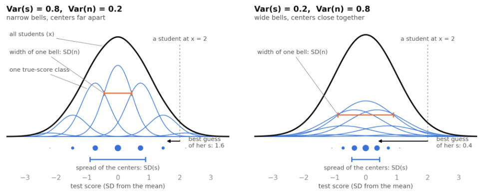
Let’s imagine each true score is a type. Students of the same type still get different scores, because each sitting draws its own error. Suppose type k has true score sks_k and makes up a fraction pkp_k of the population. Each distribution of types is the normal distribution 𝒩(sk,Var⁡(n))\mathcal{N}\big(s_k, \operatorname{Var}(n)\big). The population is their weighted sum:
f(x)=∑kpk,𝒩(sk,Var⁡(n))f(x) = \sum_k p_k , \mathcal{N}\big(s_k, \operatorname{Var}(n)\big)

The same distribution of observed scores can come from two different situations. One sitting per student cannot tell the two situations apart.

Because n is independent of s, the two variances add:

Var⁡(x)=Var⁡(s)+Var⁡(n)\operatorname{Var}(x) = \operatorname{Var}(s) + \operatorname{Var}(n)

To see why, square a student’s deviation: (s+n)2=s2+2sn+n2(s+n)^2 = s^2 + 2sn + n^2. Average each term over all students. The first gives Var(s)Var(s), and the last gives Var(n)Var(n). Inside one bell, s is fixed and n averages to zero, so the cross term 2sn2sn also averages to zero.

Because the variances add, each one is a share of the whole. The share that comes from true scores is the reliability of the test:

Reliability: λ=Var⁡(s)Var⁡(x)\text{Reliability: } \lambda = \frac{\operatorname{Var}(s)}{\operatorname{Var}(x)}

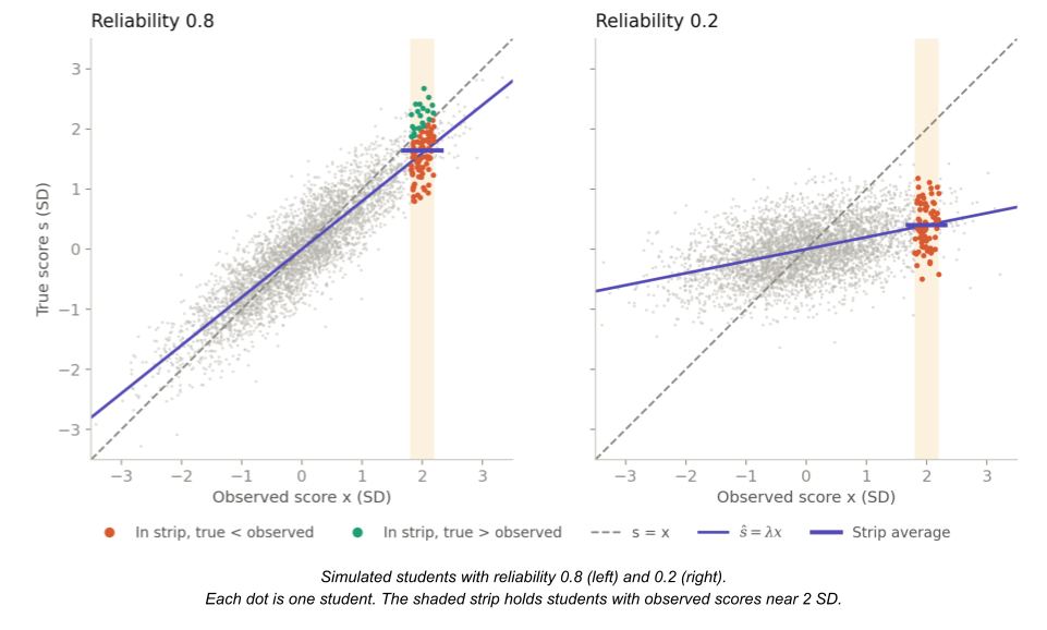
It runs from 0 to 1, and the error share is 1 − λ. In the figure, Var(x) = 1, so λ is 0.8 on the left and 0.2 on the right. So λ describes a test in one population. Give the same test to a narrower population, and Var(s) falls while Var(n) stays the same, so λ falls.

The Coefficient of Determination

Reliability answers a question: how much of the variance in observed scores does the true score predict? Regression answers the same question with the coefficient of determination.

Regress an outcome y on one predictor. The fitted line makes a prediction ŷᵢ for each observation, and the residual ei=yi−y^ieᵢ = yᵢ − ŷᵢ is the error that remains.

A model’s mean squared error (MSE) measures the performance of the model:

MSEmodel=1N∑i(yi−y^i)2=1N∑iei2\text{MSE}{\text{model}} = \frac{1}{N}\sum_i (y_i – \hat{y}i)^2 = \frac{1}{N}\sum_i e_i^2

The coefficient of determination (R²) measures how well the model’s predictions track the outcome. It compares the model’s MSE with a baseline that predicts the mean ȳ for every observation:

MSEbase=1N∑i(yi−y‾)2=Var⁡(y)\text{MSE}{\text{base}} = \frac{1}{N}\sum_i (y_i – \bar y)^2 = \operatorname{Var}(y)

R2=1−MSEmodelMSEbaseR^2 = 1 – \frac{\text{MSE}{\text{model}}}{\text{MSE}{\text{base}}}

If the model predicts every observation exactly, R² = 1. If it matches the baseline, R² = 0.

Two properties of least squares will be used in this section. First, the residuals average to zero. Second, they are uncorrelated with the predictions.

Given the first property, and the fact that a variable with zero mean has a variance equal to its mean square:

MSEmodel=1N∑iei2=Var⁡(e).\text{MSE}{\text{model}} = \frac{1}{N}\sum_i e_i^2 = \operatorname{Var}(e).

We can now write the coefficient of determination in terms of variances:

R2=1−Var⁡(e)Var⁡(y)=Var⁡(y)−Var⁡(e)Var⁡(y)R^2 = 1 – \frac{\operatorname{Var}(e)}{\operatorname{Var}(y)} = \frac{\operatorname{Var}(y) – \operatorname{Var}(e)}{\operatorname{Var}(y)}

The second property splits the variance of the outcome. Since y = ŷ + e, its variance is,

Var⁡(y^+e)=Var⁡(y^)+Var⁡(e)+2Cov⁡(y^,e)\operatorname{Var}(\hat y + e) = \operatorname{Var}(\hat y) + \operatorname{Var}(e) + 2\operatorname{Cov}(\hat y, e)

The covariance term is zero, so

Var⁡(y)=Var⁡(y^)+Var⁡(e)\operatorname{Var}(y) = \operatorname{Var}(\hat y) + \operatorname{Var}(e)

Substitute this into the numerator:

R2=Var⁡(y^)Var⁡(y)R^2 = \frac{\operatorname{Var}(\hat y)}{\operatorname{Var}(y)}

This equation is why R² is also called the explained variance.

In CTT, the noise n has both properties, so x = s + n is a least-squares regression with fit x̂ = s. We cannot run this regression, because true scores are hidden. Its R² still exists, and it is the reliability:

R2=Var⁡(x^)Var⁡(x)=Var⁡(s)Var⁡(x)=λR^2 = \frac{\operatorname{Var}(\hat x)}{\operatorname{Var}(x)} = \frac{\operatorname{Var}(s)}{\operatorname{Var}(x)} = \lambda

CTT assumes these properties. In regression, least squares provides them for the training data. On new data, the model can underperform baseline, and R² can be negative.

The Geometry of Variance

OLS Estimation via Projection showed that least squares projects a vector onto the column space of a matrix A. The residual e is perpendicular to that space: A⊤e=0A^\top e = 0. The same geometry organizes variance.

Treat each variable as a vector with one entry for each of the N students. Subtract the mean from each entry, and divide each entry by √N. The covariance is an average of products:

Cov⁡(u,v)=1N∑i=1N(ui−u‾)(vi−v‾)\operatorname{Cov}(u, v) = \frac{1}{N}\sum_{i=1}^{N} (u_i – \bar u)(v_i – \bar v)

Each vector carries a factor of 1/√N, so their dot product carries 1/N. For these vectors, statistics and geometry are related by the following identities.

Cov⁡(u,v)=u⋅v,Var⁡(u)=|u|2,σu=|u|\operatorname{Cov}(u, v) = u \cdot v, \qquad \operatorname{Var}(u) = |u|^2, \qquad \sigma_u = |u|

The correlation (r) of two variables is the covariance of their standardized versions, zu=u/σuz_u = u/\sigma_u and zv=v/σvz_v = v/\sigma_v. In vector terms, this divides the dot product by both lengths, which gives the cosine of the angle between the vectors:

Correlation: r=Cov⁡(u,v)σuσv=Cov⁡(zu,zv)=u⋅v|u|,|v|=cos⁡θ\text{Correlation: } r = \frac{\operatorname{Cov}(u, v)}{\sigma_u \sigma_v} = \operatorname{Cov}(z_u, z_v) = \frac{u \cdot v}{|u|,|v|} = \cos \theta

Two uncorrelated variables have r = 0 = cos 90°, so they are perpendicular.

Signal and noise are uncorrelated, so they are perpendicular, and x=s+nx = s + n is the hypotenuse of a right triangle. The legs have lengths σs=4\sigma_s = 4 and σn=3\sigma_n = 3, and the hypotenuse has length σx=5\sigma_x = 5. The lengths do not add: 4 + 3 ≠ 5. The areas of the squares on the sides are the variances, and they do add: 16 + 9 = 25. In this geometry, variance additivity is the Pythagorean theorem. Fisher (1918) introduced the term variance because of this additivity.
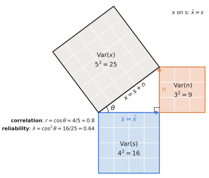
The split Var(y)=Var(y^)+Var(e)Var(y) = Var(ŷ) + Var(e) in the previous section is the same theorem. The prediction and the residual are uncorrelated, so they are perpendicular. Because the vectors are centered, a regression on one predictor projects the outcome onto the predictor.

For an outcome v and a predictor u, the residual v−buv − bu is perpendicular to u, so u·(v−bu)=0u · (v − bu) = 0. Write bv|ub_{v|u} for the slope of v on u.

bv|u=u⋅vu⋅u=Cov⁡(u,v)Var⁡(u)b_{v|u} = \frac{u \cdot v}{u \cdot u} = \frac{\operatorname{Cov}(u, v)}{\operatorname{Var}(u)}

The slope is the covariance of the predictor and the outcome, divided by the variance of the predictor. The triangle shows the regression of x on s from the previous section. The residual n is perpendicular to the predictor s, so the fit is s itself, and bx|s=1b_{x|s} = 1.
The side s is adjacent to the angle θ, and x is the hypotenuse, so

r=cos⁡θ=|s||x|=σsσx=45=0.8r = \cos \theta = \frac{\lvert s \rvert}{\lvert x \rvert} = \frac{\sigma_s}{\sigma_x} = \frac{4}{5} = 0.8

λ=R2=|s|2|x|2=cos2⁡θ=r2=1625=0.64\lambda = R^2 = \frac{|s|^2}{|x|^2} = \cos^2\theta = r^2 = \frac{16}{25} = 0.64

The reliability is the squared correlation between true and observed scores. This holds for any regression with one predictor:

R2=cos2⁡θ=r2R^2 = \cos^2\theta = r^2

Regression to the Mean

The slope of y on x is Cov(x,y)/Var(x)Cov(x, y)/Var(x). Measure both variables in standard deviations, and the slope becomes r. The slope of x on y is also r. In any units, the two slopes multiply to r²:

by|x,bx|y=Cov⁡(x,y)Var⁡(x)⋅Cov⁡(x,y)Var⁡(y)=r2b_{y|x}, b_{x|y} = \frac{\operatorname{Cov}(x,y)}{\operatorname{Var}(x)} \cdot \frac{\operatorname{Cov}(x,y)}{\operatorname{Var}(y)} = r^2

In standard units, unless the correlation is exact, every prediction is less extreme than its predictor. Galton (1886) found this in human stature. He compared the heights of children with the mean height of their parents and found a slope of about two thirds: parents whose mean height is 3 inches above average have children about 2 inches above average. He called this effect regression towards mediocrity. We now call it regression to the mean.

The slope of about two thirds is measured in inches per inch. It differs from the correlation because parental averages vary less than children’s heights.
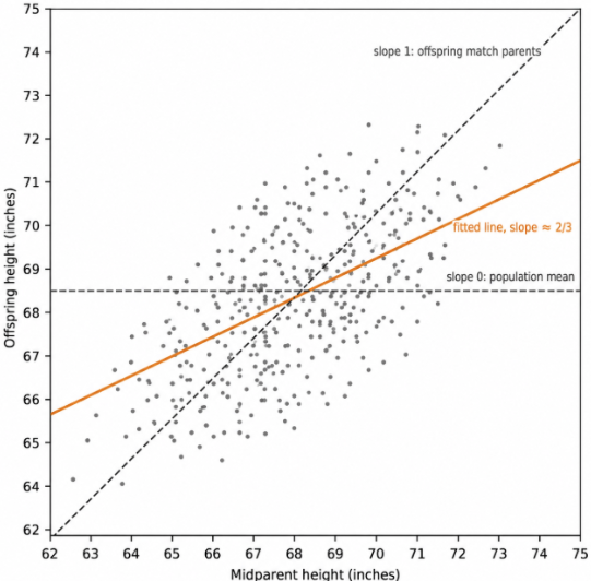
Regression to the mean also runs backward in time: tall children have parents who are, on average, less tall than they are. The effect doesn’t require a causal mechanism. It manifests whenever measurements share a signal but also draw independent noise.

When a test is administered twice, for example, the two sittings share a true score and nothing else, so their covariance is Var(s). They also have the same variance, Var(x). So the slope of retest on test and their correlation are both Var(s)/Var(x)=λVar(s)/Var(x) = λ.

Galton’s data has the same structure. The mid-parent height is a noisy measure of the parents’ mean additive genetic value: the part of genetic value that children inherit on average. A child inherits that value and draws new noise of its own. So the covariance of child and mid-parent is the variance of the genetic signal, and the slope of child on mid-parent is a reliability ratio. The child’s height varies more than the mid-parent’s, so here only the slope equals this ratio. Quantitative genetics calls this ratio heritability. Under simple genetic assumptions, Galton’s slope of about two thirds measures the heritability of height.

Reliability is the slope of retest on test. It is the component of a result that carries over to the next measurement.

Shrinkage

Recall our student with a strong test score. Regression to the mean says her retest will probably be lower. What is her true score?
The geometry section knew the true score (s) and predicted the observed score (x). It regressed x on s. Our student’s case runs the other way. We know only her observed score, so we regress s on x to estimate her true score.

Independent noise adds nothing to a covariance, so the covariance of the true and observed scores is the variance of the signal:
Cov⁡(s,x)=Var⁡(s)\operatorname{Cov}(s, x) = \operatorname{Var}(s)

A slope is this covariance divided by the variance of the predictor, so only the denominator changes:

bx|s=Var⁡(s)Var⁡(s)=1,bs|x=Var⁡(s)Var⁡(x)=λb_{x|s} = \frac{\operatorname{Var}(s)}{\operatorname{Var}(s)} = 1, \qquad b_{s|x} = \frac{\operatorname{Var}(s)}{\operatorname{Var}(x)} = \lambda

If we know a student’s true score, her observed score averages to that true score. When true scores and errors are normal, no curve does better than the line ŝ = λx. This estimate is called Kelley’s rule. Kelley (1927) derived it in the context of test scores. It is a weighted average of the test score X and the population mean μ:

s^raw=λX+(1−λ)μ\hat{s}_{\text{raw}} = \lambda X + (1-\lambda)\mu

If the test has high reliability, the estimator trusts the score. Else, it trusts the population mean.

Consider students who achieve a test score of 2 SD. By definition of the normal distribution, many of these students have a true score near 1 SD. So an observed score of 2 SD comes more often from a good student with good luck than from an excellent student with average luck. Consider one of these students. Reliability tells us how much of her lead is skill. With a reliability of 0.8, about 80% of her 2 SD lead is skill, so her best-guess true score is about 1.6 SD.
A Kalman filter (Kalman 1960) tracks a hidden quantity with a current estimate. The estimate’s error has variance P, and each measurement adds noise with variance R. These play the same roles of Var(s) and Var(n) in CTT. The estimate has variance P + R. The filter moves its estimate toward the measurement by a weight K called the gain:

K=Var⁡(true step)Var⁡(measured step)=PP+RK = \frac{\operatorname{Var}(\text{true step})}{\operatorname{Var}(\text{measured step})} = \frac{P}{P + R}

The Kalman filter uses Kelley’s rule, but with the current estimate in place of the population mean. A noisy measurement has a small gain and is largely ignored.

Reliability is also a shrinkage factor. It is the share of an observed lead that we credit to the true score.

Attenuated Slopes

The true scores are often latent, but estimating them can enable downstream predictions. An epidemiologist wants to know how much stroke risk rises with blood pressure. She needs the slope of stroke risk y on each patient’s usual blood pressure s. But she has only one reading x per patient, a noisy measure of s. If she regresses stroke risk on the readings, what slope does she get?

Suppose an outcome depends on the true score, y=βs+εy = βs + ε. The slope we want is by|s=βb_{y|s} = \beta. True scores are hidden, so we can fit only by|x b_{y|x}, the regression of y on the observed score x = s + n. Write λx\lambda_x for the reliability of x.

x=s+n,y=βs+ε,by|x=Cov⁡(y, x)Var⁡(x)=Cov⁡(βs+ε, s+n)Var⁡(x)x = s + n,\quad y = \beta s + \varepsilon,\quad b_{y|x} = \frac{\operatorname{Cov}(y,\ x)}{\operatorname{Var}(x)} = \frac{\operatorname{Cov}(\beta s + \varepsilon,\ s + n)}{\operatorname{Var}(x)}

If we assume the noise n and the error ε are independent of s and of each other, they add nothing to the covariance:

Cov⁡(βs+ε, s+n)=βVar⁡(s)+βCov⁡(s,n)+Cov⁡(ε,s)+Cov⁡(ε,n)=βVar⁡(s)\operatorname{Cov}(\beta s + \varepsilon,\ s + n) = \beta\operatorname{Var}(s) + \beta\operatorname{Cov}(s, n) + \operatorname{Cov}(\varepsilon, s) + \operatorname{Cov}(\varepsilon, n) = \beta\operatorname{Var}(s)

by|x=Cov⁡(βs+ε, s+n)Var⁡(x)=β,Var⁡(s)Var⁡(x)=by|s,bs|x=βλxb_{y|x} = \frac{\operatorname{Cov}(\beta s + \varepsilon,\ s + n)}{\operatorname{Var}(x)} = \beta,\frac{\operatorname{Var}(s)}{\operatorname{Var}(x)} = b_{y|s}, b_{s|x} = \beta\lambda_x

The slope from a noisy predictor is a product of two factors. The first shrinks the observed score to estimated true score by the reliability. The second factor β carries the true score to the outcome. This process is known as attenuation bias, or regression dilution.
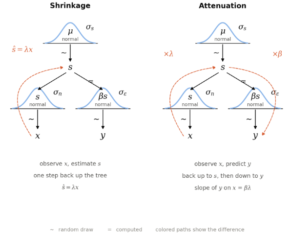
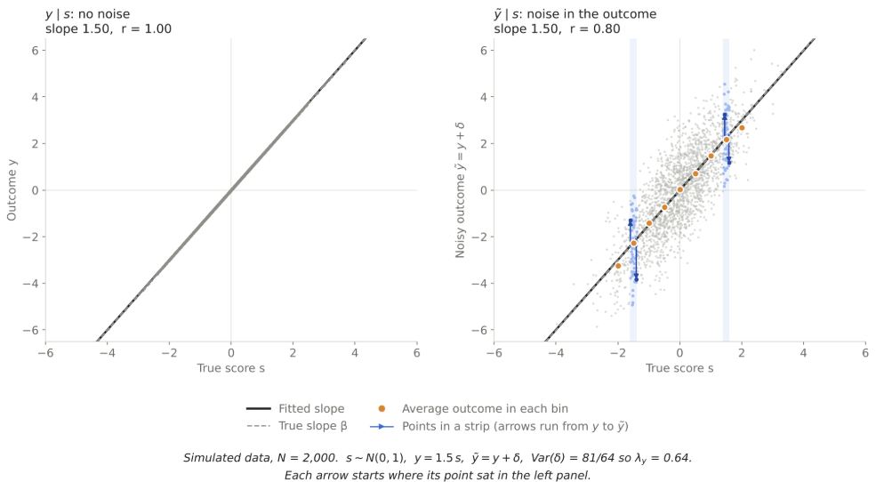
An illustration of the shrinkage. Adding noise to the predictor is visualized as horizontal arrows. The slope of the estimated function flattens.
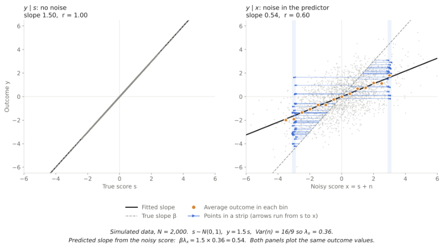
Her slope from the readings is βλx\beta\lambda_x. For predicting stroke from one reading, this is the best slope she can use. To recover β itself, she divides her slope by λx\lambda_x, which she can estimate from repeated readings on some of her patients. MacMahon et al. (1990) made this correction in studies of blood pressure and heart disease. The corrected associations with stroke and coronary heart disease were about 60% stronger than the uncorrected ones.

A related effect appears in models trained on many features. Suppose the model also sees a feature z that correlates with the true score s. Then z takes over part of the weight that x loses, even if z has no effect on the outcome. If s is a confounder, epidemiologists call the bias that remains after adjusting for x residual confounding (Phillips & Davey Smith 1991).

Attenuated Correlations

Suppose we score a model against labels from one radiologist. The labels are a noisy measure of the true outcome. Write the radiologist’s label as

y~=y+δ\tilde{y} = y + \delta

where δ is the radiologist’s error, independent of s, n, and ε. How does label noise change the slope and the correlation?

In the algebra, δ adds nothing to the covariance, so the slope is unchanged:

by~|x=Cov⁡(y+δ, x)Var⁡(x)=Cov⁡(y, x)Var⁡(x)=by|xb_{\tilde y|x} = \frac{\operatorname{Cov}(y + \delta,\ x)}{\operatorname{Var}(x)} = \frac{\operatorname{Cov}(y,\ x)}{\operatorname{Var}(x)} = b_{y|x}

But the noisy label does attenuate the correlation. Recall our definitions.

rtrue=Cov⁡(s, y)σs,σy,robserved=Cov⁡(x, y~)σx,σy~r_{\text{true}} = \frac{\operatorname{Cov}(s,\ y)}{\sigma_s,\sigma_y}, \qquad r_{\text{observed}} = \frac{\operatorname{Cov}(x,\ \tilde y)}{\sigma_x,\sigma_{\tilde y}}

λx=Var(s)Var(x),λx=σsσx,λy=Var(y)Var(y~),λy=σyσy~\lambda_x = \frac{\mathrm{Var}(s)}{\mathrm{Var}(x)}, \qquad \sqrt{\lambda_x} = \frac{\sigma_s}{\sigma_x}, \qquad \lambda_y = \frac{\mathrm{Var}(y)}{\mathrm{Var}(\tilde{y})}, \qquad \sqrt{\lambda_y} = \frac{\sigma_y}{\sigma_{\tilde y}}

The noises are independent, so the numerators are equal.

Cov⁡(x, y~)=Cov⁡(s+n, y+δ)=Cov⁡(s, y)\operatorname{Cov}(x,\ \tilde y) = \operatorname{Cov}(s + n,\ y + \delta) = \operatorname{Cov}(s,\ y)

Multiply the true correlation by a ratio of standard deviations to get the observed correlation:

rtrueσsσyσxσy~=Cov(s,y)σsσy⋅σsσyσxσy~=Cov(x,y~)σxσy~=robservedr_{\text{true}} \frac{\sigma_s \sigma_y}{\sigma_x \sigma_{\tilde y}} = \frac{\mathrm{Cov}(s, y)}{\sigma_s \sigma_y} \cdot \frac{\sigma_s \sigma_y}{\sigma_x \sigma_{\tilde y}} = \frac{\mathrm{Cov}(x, \tilde y)}{\sigma_x \sigma_{\tilde y}} = r_{\text{observed}}

Both reliability ratios reduce the correlation, so observed correlations are closer to zero than true correlations.

robserved=rtrueσsσxσyσy~=rtrue(λxλy1/2)r_{\text{observed}} = r_{\text{true}} \frac{\sigma_s}{\sigma_x} \frac{\sigma_y}{\sigma_{\tilde y}} = r_{\text{true}} {(\lambda_x \lambda_y}^{1/2})

Spearman (1904) named this weakening attenuation. To correct an observed correlation, divide it by(λxλy)1/2 (\lambda_x \lambda_y)^{1/2}.

In the figure, the left panel has no noise. In the right panel, each point moves up or down by its noise, and its true score stays the same. The noise averages to zero in each bin, so the orange dots stay on the true line, and the slope stays at 1.5. The correlation falls from 1 to λy1/2=0.8{\lambda_y}^{1/2} = 0.8.

These are the regressions of this post, each with its slope and correlation.
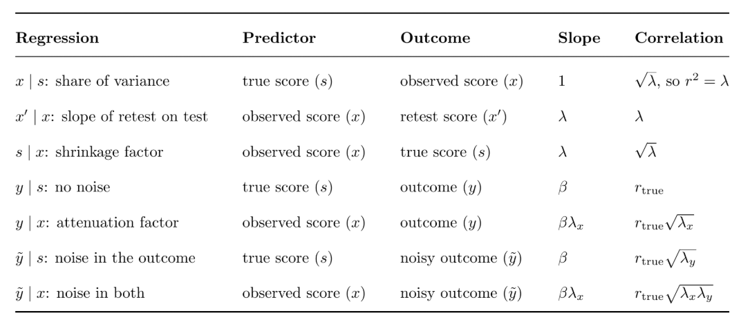
Reliability is also an attenuation factor. A noisy predictor keeps the share λ of a true slope, and each noisy measurement keeps the share √λ of a true correlation.

Estimating Reliability

So far, we have treated the reliability λ as known. In practice, we must estimate it. One score per student cannot provide an estimate, but a second score of the same student can. Since test and retest share the true score and nothing else, we saw that their correlation was λ. More sittings give a better estimate of λ, and their average is a more reliable score.

Suppose each of N students sits the test m times. The score of student i on sitting j, and her average across all sittings are:

xij=si+nij,x‾i=si+n‾ix_{ij} = s_i + n_{ij}, \qquad \bar{x}_i = s_i + \bar{n}_i

The true score and the errors are independent, so their variances add

Var⁡(x‾i)=Var⁡(s)+Var⁡(n‾i)=Var⁡(s)+Var⁡(n)m\operatorname{Var}(\bar{x}_i) = \operatorname{Var}(s) + \operatorname{Var}(\bar{n}_i) = \operatorname{Var}(s) + \frac{\operatorname{Var}(n)}{m}

Across m sittings, the reliability of the average λm\lambda_m is the share of this variance that comes from the true score.

λm=Var⁡(s)Var⁡(x‾i)=Var⁡(s)Var⁡(s)+Var⁡(n)/m\lambda_m = \frac{\operatorname{Var}(s)}{\operatorname{Var}(\bar{x}_i)} = \frac{\operatorname{Var}(s)}{\operatorname{Var}(s) + \operatorname{Var}(n)/m}

For one sitting, recall the signal share and error share:

λ=Var⁡(s)Var⁡(x)1−λ=Var⁡(n)Var⁡(x)\lambda = \frac{\operatorname{Var}(s)}{\operatorname{Var}(x)} \qquad 1-\lambda = \frac{\operatorname{Var}(n)}{\operatorname{Var}(x)}

The relationship between reliability of the average and single-sitting reliability is known as the Spearman-Brown formula (Spearman 1910; Brown 1910).
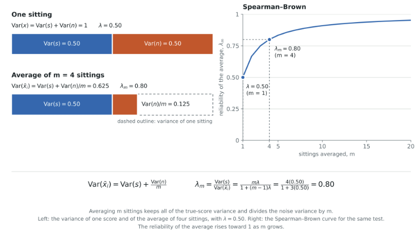
λm=mλ1+(m−1)λ\lambda_m = \frac{m\lambda}{1 + (m-1)\lambda}

Repeated sittings also let us estimate the signal and noise variances. The spread of each student’s scores around her own average estimates Var(n). The spread of the student averages around the grand average x̄, the average of all the scores, estimates Var(x̄ᵢ). We write these estimates as σ̂²ₙ and σ̂²ₓ̄:

σ^n2=1N(m−1)∑i=1N∑j=1m(xij−x‾i)2σ^x‾2=1N−1∑i=1N(x‾i−x‾)2\hat{\sigma}^2_n = \frac{1}{N(m-1)} \sum_{i=1}^{N} \sum_{j=1}^{m} \left(x_{ij} – \bar{x}_i\right)^2 \qquad \hat{\sigma}^2_{\bar{x}} = \frac{1}{N-1} \sum_{i=1}^{N} \left(\bar{x}_i – \bar{x}\right)^2

These divisors differ from the 1/N of earlier sections. Scores sit closer to their own average than to their true mean, so dividing by the number of scores would give too small an estimate. Each divisor counts degrees of freedom: m – 1 inside each of the N students, and N – 1 for the averages.

Replace each variance in the equation for the variance of the average with its estimate, solve for the signal variance, and substitute the estimates into both reliabilities:

σ^s2=σ^x‾2−σ^n2mλ^=σ^s2σ^s2+σ^n2λ^m=σ^s2σ^s2+σ^n2/m\hat{\sigma}^2_s = \hat{\sigma}^2_{\bar{x}} – \frac{\hat{\sigma}^2_n}{m} \qquad \hat{\lambda} = \frac{\hat{\sigma}^2_s}{\hat{\sigma}^2_s + \hat{\sigma}^2_n} \qquad \hat{\lambda}_m = \frac{\hat{\sigma}^2_s}{\hat{\sigma}^2_s + \hat{\sigma}^2_n / m}

Thus, the Spearman–Brown formula can be applied to estimate λ and λm\lambda_m.

This method is the analysis of variance (ANOVA), and Hoyt (1941) used it to estimate reliability. ANOVA states both spreads on the scale of one sitting, as the mean square within (MSW) and the mean square between (MSB).

MSW=σ^n2MSB=mσ^x‾2\text{MSW} = \hat{\sigma}^2_n \qquad \text{MSB} = m \hat{\sigma}^2_{\bar{x}}

More sittings make the noise estimate precise. Only more students make the signal estimate precise, because the spread of the averages has N-1 degrees of freedom. With a reliability of 0.8, a second sitting for every student raises the effective sample size by about 11%, and a second set of students raises it by 100%. Extra sittings pay off only when the averaged score is still noisy or when new students are expensive to recruit.

A retest needs a second sitting. Cronbach’s alpha (Cronbach 1951) estimates reliability from one sitting. Each question acts as a short retest of the same true score. So each covariance between two questions estimates the signal variance, and each question’s variance estimates the variance of one score. The average covariance c over the average variance v then estimates the reliability of one question. This estimate assumes that every question measures the true score equally strongly. The m questions play the role of m sittings, and the total score has the same reliability as their average. So the Spearman–Brown formula gives alpha:

α=m,c/v1+(m−1),c/v=m,cv+(m−1),c\alpha = \frac{m,c/v}{1 + (m-1),c/v} = \frac{m,c}{v + (m-1),c}

Psychometricians use alpha to build tests: they keep the questions that raise alpha and drop the ones that lower it.

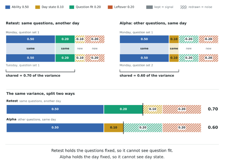
The two formulas average over different replications. For reliability of the average, the replications are m sittings of the same test on different days. For alpha, they are the m questions of one sitting. Retest reliability and Cronbach’s alpha can differ for the same test. A more granular analysis of variance explains the divergence. Divide each score into four parts:

  • Ability (e.g., intelligence)
  • Day state (e.g., sleep or mood)
  • Question fit (e.g., having studied these topics)
  • Leftover (e.g., a lucky guess)

Administering a test again on a different day keeps only ability and question fit. Administering different questions in one sitting retains ability and day state. This approach to variance is further elaborated in generalizability theory (Cronbach et al. 1972).
Hierarchical Models

CTT has two levels: students taking multiple tests (i.e., sittings). A hierarchical model (HM) has two levels, but at a different granularity: groups having multiple members. In HM, each score is an observation of the group mean. Sittings are glossed over as part of the individual variance.
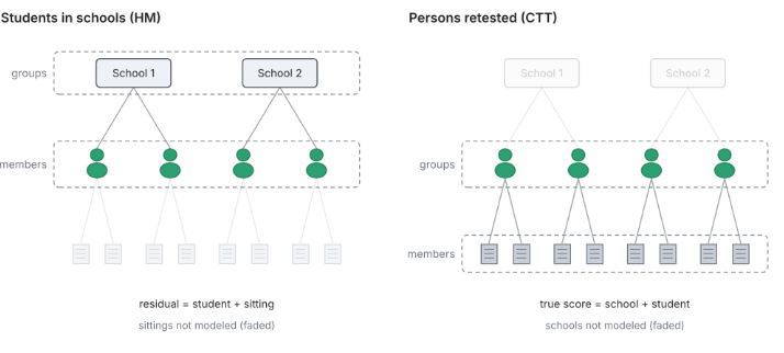
Many of our CTT constructs reappear in HM with new labels.
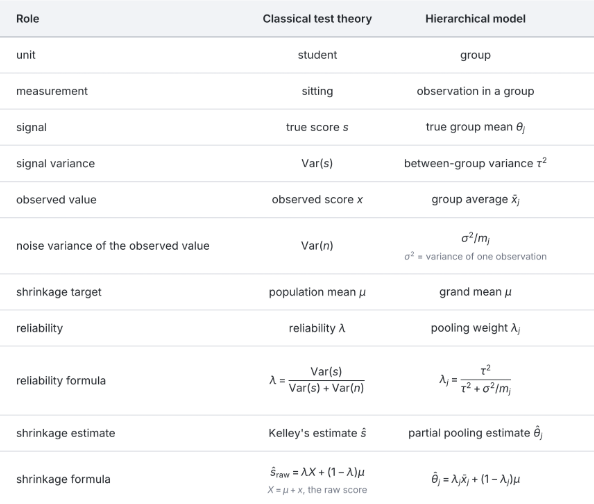
CTT gives every student the same number of sittings, but HM lets groups differ in size. Let mⱼ be the number of students in school j. A school with 20 students and a school with 2,000 students might each report average test scores, and the score of the former is much noisier. Let τ² denote the variance of the true group scores, and σ² denote the variance of student scores within the school. The Spearman–Brown formula gives the reliability of each school:

λj=τ2τ2+σ2/mj\lambda_j = \frac{\tau^2}{\tau^2 + \sigma^2/m_j}

The estimate of each group mean is Kelley’s rule, with the grand mean μ in place of the population mean:

θ^j=λj,x‾j+(1−λj),μ\hat{\theta}_j = \lambda_j,\bar{x}_j + (1-\lambda_j),\mu

Statisticians call this estimate partial pooling. It is a compromise between no pooling (each school keeps its own score) and complete pooling (every group is estimated with the grand mean). Each estimate θ̂ⱼ depends on τ², σ², and μ, and all three come from every group. So each estimate uses information from the other groups. This is known as borrowing strength.

With equal sizes, one weight scales every average, and the rank order stays the same. With unequal sizes, small groups move further toward the grand mean than large groups, so groups can change rank. Wainer (2007) described a case from education. Small schools were overrepresented among the schools with the highest test scores, and this result encouraged large investments in smaller schools. Small schools were also overrepresented among the schools with the lowest scores.

Wainer named the rule behind this pattern de Moivre’s equation: the error of an average of m observations has standard deviation σ/√m. A small school averages few students, so its average has a large error. Large errors put small schools in both tails. The same rule puts small units in both tails in other domains. The US counties with the highest and the lowest kidney cancer death rates are mostly small rural counties (Gelman & Price 1999). Hospitals that treat few patients have the most extreme death rates (Spiegelhalter 2005). Products with few reviews fill both ends of rating lists. Partial pooling moves these small units toward the grand mean.
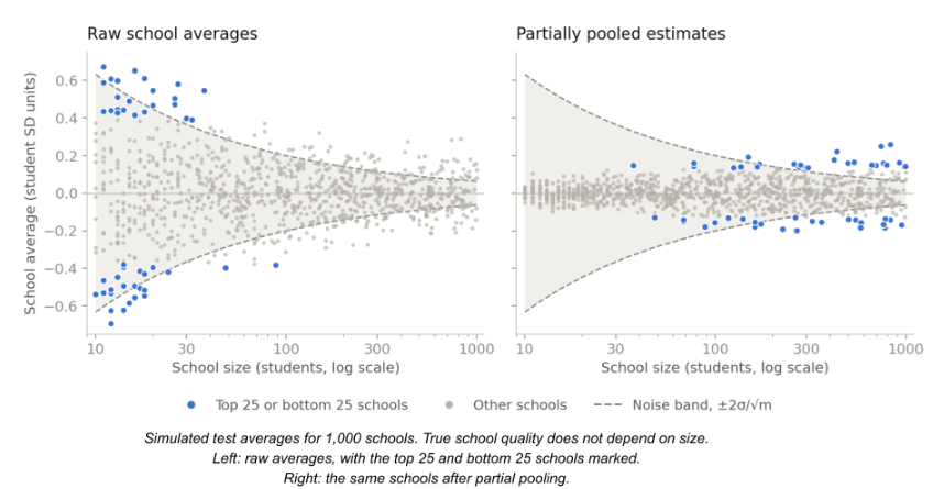
In the left panel, all 50 of the most extreme schools have fewer than 100 students. In the right panel, the extremes are now mostly large schools.

Reliability is also a pooling weight. It is the share of its own average that each group keeps.

Reliability and Regularization

Intro to Regularization added a penalty on the size of a model’s weights. With standardized and uncorrelated features, this ridge penalty shrinks each least-squares weight toward zero by a factor with the same form as the reliability ratio (Hastie et al. 2009). An unregularized fit corresponds to perfect reliability, taking the data at face value. Training on inputs with added noise has the same effect as ridge regression for linear models (Bishop 1995), so attenuation is also a form of regularization.

Maximum likelihood estimation (MLE) estimates each mean by its observed value. But noise accumulates, and the estimate vector is too long on average. Stein (1956) showed that for three or more means, the MLE is inadmissible: another estimator has lower expected total squared error for every possible set of true means. The means can be unrelated, which is why the result is called Stein’s paradox. James & Stein (1961) gave such an estimator. It pulls every estimate toward zero by one shared reliability factor: the share of the estimates’ squared size that comes from the true means.

Model selection compares candidate models and keeps the one with the best score. Any score used to make this choice is optimistic. The winner probably had good luck on the scoring data, and its score will probably decrease on fresh data. This phenomenon of selection bias (Cawley & Talbot 2010) is another form of regression to the mean. Bidders in auctions call it the winner’s curse (Capen et al. 1971). Data partitioning creates a retest. An untouched holdout set draws fresh luck, so its score is honest.

Wrapping Up

The reliability λ plays five roles:
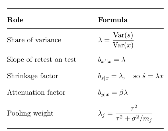
References

  • Bishop (1995). Training with noise is equivalent to Tikhonov regularization.
  • Brown (1910). Some experimental results in the correlation of mental abilities.
  • Capen, Clapp & Campbell (1971). Competitive bidding in high-risk situations.
  • Cawley & Talbot (2010). On over-fitting in model selection and subsequent selection bias in performance evaluation.
  • Cronbach (1951). Coefficient alpha and the internal structure of tests.
  • Cronbach et al. (1972). The Dependability of Behavioral Measurements.
  • Fisher (1918). The correlation between relatives on the supposition of Mendelian inheritance.
  • Galton (1886). Regression towards mediocrity in hereditary stature.
  • Gelman & Price (1999). All maps of parameter estimates are misleading.
  • Hastie, Tibshirani & Friedman (2009). The Elements of Statistical Learning.
  • Hoyt (1941). Test reliability estimated by analysis of variance.
  • James & Stein (1961). Estimation with quadratic loss.
  • Kalman (1960). A new approach to linear filtering and prediction problems.
  • Kelley (1927). Interpretation of Educational Measurements.
  • MacMahon et al. (1990). Blood pressure, stroke, and coronary heart disease. Part 1, prolonged differences in blood pressure: prospective observational studies corrected for the regression dilution bias.
  • Phillips & Davey Smith (1991). How independent are “independent” effects? Relative risk estimation when correlated exposures are measured imprecisely.
  • Spearman (1904). The proof and measurement of association between two things.
  • Spearman (1910). Correlation calculated from faulty data.
  • Spiegelhalter (2005). Funnel plots for comparing institutional performance.
  • Stein (1956). Inadmissibility of the usual estimator for the mean of a multivariate normal distribution.
  • Wainer (2007). The most dangerous equation.

The Last Bits are Deepest

Part Of: Machine Learning sequence
Content Summary: 2000 words, 10min read. 
Excerpt 1 From: The Unreasonable Effectiveness of Recurrent Neural Networks
Excerpt 2 From: The Scaling Hypothesis

How Much Money Is It Worth?

A language model computes the probability of the next word, given some set of tokens. Individual predictions are optimized using cross-entropy loss, to increase the weight given the correct prediction. For example, this toy model fails to assign much probability to the word “train”, so its loss is 2.69.  

In a real language model, probability mass is spread across all possible outputs – the entire vocabulary.  On the very first prediction, the model will judge every output equally likely. For a 10k word vocabulary, you would expect the cross-entropy loss to start at approximately -ln(1/10000) ≈ 9.21. From this starting point, loss will drop to some loss floor, e.g. 4 nats/token. 

The loss floor can change as a function of dataset size, model complexity, and available compute. With the discovery of neural scaling laws, we can predict how much loss that a compute budget can achieve. Research project sized budgets (e.g., $10k) can achieve a loss floor of 2.2. But in the era of large language models (LLMs), we have spent $400m to achieve a loss of 1.2. In contrast, humans can only achieve a loss of 1.7 on familiar texts. 

But what exactly is gained from building a model with 0.5 fewer nats per token (NPT)? Is 1.2 NPT really worth the $400m it takes to train it? 

To answer this, let’s explore what a model learns across different loss regimes.

Excerpt 1: Sampling Char-RNNs Output

This passage comes from: The Unreasonable Effectiveness of Recurrent Neural Networks

It’s fun to look at how the sampled text evolves while the model trains. For example, I trained an LSTM of Leo Tolstoy’s War and Peace and then generated samples every 100 iterations of training. At iteration 100 the model samples random jumbles:

tyntd-iafhatawiaoihrdemot  lytdws  e ,tfti, astai f ogoh eoase rrranbyne ‘nhthnee e plia tklrgd t o idoe ns,smtt   h ne etie h,hregtrs nigtike,aoaenns lng

However, notice that at least it is starting to get an idea about words separated by spaces. Except sometimes it inserts two spaces. It also doesn’t know that comma is almost always followed by a space. At 300 iterations we see that the model starts to get an idea about quotes and periods:

“Tmont thithey” fomesscerliund Keushey. Thom here sheulke, anmerenith ol sivh I lalterthend Bleipile shuwy fil on aseterlome coaniogennc Phe lism thond hon at. MeiDimorotion in ther thize.”

The words are now also separated with spaces and the model starts to get the idea about periods at the end of a sentence. At iteration 500:

we counter. He stutn co des. His stanted out one ofler that concossions and was to gearang reay Jotrets and with fre colt otf paitt thin wall. Which das stimn 

The model has now learned to spell the shortest and most common words such as “we”, “He”, “His”, “Which”, “and”, etc. At iteration 700 we’re starting to see more and more English-like text emerge:

Aftair fall unsuch that the hall for Prince Velzonski’s that me of her hearly, and behs to so arwage fiving were to it beloge, pavu say falling misfort how, and Gogition is so overelical and ofter.

At iteration 1200 we’re now seeing use of quotations and question/exclamation marks. Longer words have now been learned as well:

“Kite vouch!” he repeated by her door. “But I would be done and quarts, feeling, then, son is people….”

Until at last we start to get properly spelled words, quotations, names, and so on by about iteration 2000:

“Why do what that day,” replied Natasha, and wishing to himself the fact the princess, Princess Mary was easier, fed in had oftened him. Pierre aking his soul came to the packs and drove up his father-in-law women.

The picture that emerges is that the model first discovers the general word-space structure and then rapidly starts to learn the words; First starting with the short words and then eventually the longer ones. Topics and themes that span multiple words (and in general longer-term dependencies) start to emerge only much later.

Excerpt 2: Learning Trickles Up the Abstraction Hierarchy

This passage is modified from: The Scaling Hypothesis. I converted his bits per character (BPC) into nats per token (NPT) using a 4ln2 conversion factor. 

Early on in training, a model learns the crudest levels: that some letters like ‘e’ are more frequent than others like ‘z’, that every 5 characters or so there is a space, and so on. It goes from predicted uniformly-distributed bytes to what looks like Base-60 encoding—alphanumeric gibberish. As crude as this may be, it’s enough to make quite a bit of absolute progress: a random predictor needs 8 bits to ‘predict’ a byte/character, but just by at least matching letter and space frequencies, it can almost halve its error. Because it is learning so much from every character, and because the learned frequencies are simple, it can happen so fast that if one is not logging samples frequently, one might not even observe the improvement.

As training progresses, the task becomes more difficult. Now it begins to learn what words actually exist and do not exist. It doesn’t know anything about meaning, but at least now when it’s asked to predict the second half of a word, it can actually do that to some degree, saving it a few more bits. This takes a while because any specific instance will show up only occasionally: a word may not appear in a dozen samples, and there are many thousands of words to learn. With some more work, it has learned that punctuation, pluralization, possessives are all things that exist. Put that together, and it may have progressed again, all the way down to 8 NPT! (While the progress is gratifyingly fast, it’s still all gibberish, though, makes no mistake: a sample may be spelled correctly, but it doesn’t make even a bit of sense.)

But once a model has learned a good English vocabulary and correct formatting/spelling, what’s next? There’s not much juice left in predicting within-words. The next thing is picking up associations among words. What words tend to come first? What words ‘cluster’ and are often used nearby each other? Nautical terms tend to get used a lot with each other in sea stories, and likewise Bible passages, or American history Wikipedia article, and so on. If the word “Jefferson” is the last word, then “Washington” may not be far away, and it should hedge its bets on predicting that ‘W’ is the next character, and then if it shows up, go all-in on “ashington”. Such bag-of-words approaches still predict badly, but now we’re down to perhaps 7 NPT.

What next? Does it stop there? Not if there is enough data and the earlier stuff like learning English vocab doesn’t hem the model in by using up its learning ability. Gradually, other words like “President” or “general” or “after” begin to show the model subtle correlations: “Jefferson was President after…” With many such passages, the word “after” begins to serve a use in predicting the next word, and then the use can be broadened.

By this point, the loss is perhaps 6 NPT: every additional 0.1 decrease comes at a steeper cost and takes more time. However, now the sentences have started to make sense. A sentence like “Jefferson was President after Washington” does in fact mean something (and if occasionally we sample “Washington was President after Jefferson”, well, what do you expect from such an un-converged model). Jarring errors will immediately jostle us out of any illusion about the model’s understanding, and so training continues. (Around here, Markov chain & n–gram models start to fall behind; they can memorize increasingly large chunks of the training corpus, but they can’t solve increasingly critical syntactic tasks like balancing parentheses or quotes, much less start to ascend from syntax to semantics.)

Now training is hard. Even subtler aspects of language must be modeled, such as keeping pronouns consistent. This is hard in part because the model’s errors are becoming rare, and because the relevant pieces of text are increasingly distant and ‘long-range’. As it makes progress, the absolute size of errors shrinks dramatically. Consider the case of associating names with gender pronouns: the difference between “Janelle ate some ice cream, because he likes sweet things like ice cream” and “Janelle ate some ice cream, because she likes sweet things like ice cream” is one no human could fail to notice, and yet, it is a difference of a single letter. If we compared two models, one of which didn’t understand gender pronouns at all and guessed ‘he’/‘she’ purely at random, and one which understood them perfectly and always guessed ‘she’, the second model would attain a lower average error of barely <0.05 NPT!

Nevertheless, as training continues, these problems and more, like imitating genres, get solved, and eventually at a loss of 3-5 (where a small char-RNN might converge on a small corpus like Shakespeare or some Project Gutenberg ebooks), we will finally get samples that sound human—at least, for a few sentences. These final samples may convince us briefly, but, aside from issues like repetition loops, even with good samples, the errors accumulate: a sample will state that someone is “alive” and then 10 sentences later, use the word “dead”, or it will digress into an irrelevant argument instead of the expected next argument, or someone will do something physically improbable, or it may just continue for a while without seeming to get anywhere.

The pretraining thesis argues that this can go even further: we can compare this performance directly with humans doing the same objective task, who can achieve closer to 2 NPT⁠. What is in that missing 1.0 NPT?

Well—everything! Everything that the model misses. While just babbling random words was good enough at the beginning, at the end, it needs to be able to reason our way through the most difficult textual scenarios requiring causality or commonsense reasoning. Every error where the model predicts that ice cream put in a freezer will “melt” rather than “freeze”, every case where the model can’t keep straight whether a person is alive or dead, every time that the model chooses a word that doesn’t help build somehow towards the ultimate conclusion of an ‘essay’, every time that it lacks the theory of mind to compress novel scenes describing the Machiavellian scheming of a dozen individuals at dinner jockeying for power as they talk, every use of logic or abstraction or instructions or Q&A where the model is befuddled and needs more bits to cover up for its mistake where a human would think, understand, and predict. For a language model, the truth is that which keeps on predicting well—because truth is one and error many. Each of these cognitive breakthroughs allows ever so slightly better prediction of a few relevant texts; nothing less than true understanding will suffice for ideal prediction.

If we trained a model which reached that loss of <2.0, which could predict text indistinguishable from a human, whether in a dialogue or quizzed about ice cream or being tested on SAT analogies or tutored in mathematics, if for every string the model did just as good a job of predicting the next character as you could do, how could we say that it doesn’t truly understand everything? (If nothing else, we could, by definition, replace humans in any kind of text-writing job!)

The last bits are deepest. The implication here is that the final few bits are the most valuable bits, which require the most of what we think of as intelligence. A helpful analogy here might be our actions: for the most part, all humans execute actions equally well. We all pick up a tea mug without dropping, and can lift our legs to walk down thousands of steps without falling even once. For everyday actions (the sort which make up most of a corpus), anybody, of any intelligence, can get enough practice & feedback to do them quite well, learning individual algorithms to solve each class of problems extremely well, in isolation. Meanwhile for rare problems, there may be too few instances to do any better than memorize the answer. In the middle of the spectrum are problems which are similar but not too similar to other problems; these are the sorts of problems which reward flexible meta-learning and generalization, and many intermediate problems may be necessary to elicit those capabilities.

Regression vs Classification

Part Of: Machine Learning sequence
Content Summary: 500 words, 5 min read

Motivations

Data scientists are in the business of answering questions with data. To do this, data is fed into prediction functions, which learn from the data, and use this knowledge to produce inferences.

Today we take an intuitive, non-mathematical look at two genres of prediction machine: regression and classification. Whereas these approaches may seem unrelated, we shall discover a deep symmetry lurking below the surface.

Introducing Regression

Consider a supermarket that has made five purchases of sugar from its supplier in the past. We therefore have access to five data points:

Regression Classification- Regression Data (3)

One of our competitors intends to buy 40kg of sugar. Can we predict the price they will pay?

This question can be interpreted visually as follows:

Regression Classification- Regression Prediction Visualization

But there is another, more systematic way to interpret this request. We can differentiate training data (the five observations where we know the answer) versus test data (where we are given a subset of the relevant information, and asked to generate the rest):

Regression Classification- Regression Prediction Schema

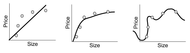
A regression prediction machine will for any hypothetical x-value, predicts the corresponding y-value. Sound familiar? This is just a function. There are in fact many possible regression functions, of varying complexity:

Regression Classification- Simple vs Complex Regression Outputs

Despite their simple appearance, each line represents a complete prediction machine. Each one can, for any order size, generate a corresponding prediction of the price of sugar.

Introducing Classification

To illustrate classification, consider another example.

Suppose we are an animal shelter, responsible for rescuing stray dogs and cats. We have saved two hundred animals; for each, we record their height, weight, and species:
Regression Classification- Classification Data (1)

Suppose we are left a note that reads as follows:

I will be dropping off a stray tomorrow that is 19 lbs and about a foot tall.

A classification question might be: is this animal more likely to be a dog or a cat?

Visually, we can interpret the challenge as follows:

Regression Classification- Classification Prediction Interpretation (2)

As before, we can understand this prediction problem as taking information gained from training data, to generate “missing” factors” from test data:

Regression Classification- Classification Prediction Schema

To actually build a classification machine, we must specify a region-color map, such as the following:

Regression Classification- Simple Classification Output

Indeed, the above solution is complete: we can produce a color (species) label for any new observation, based on whether it lies above or below our line. 

But other solutions exist. Consider, for example, a rather different kind of map:Regression Classification- Complex Classification Boundary

We could use either map to generate predictions. Which one is better? We will explore such questions next time.

Comparing Prediction Methods

Let’s compare our classification and regression models. In what sense are they the same?

Regresssion Classification- Comparing Models

If you’re like me, it is hard to identify similarities. But insight is obtained when you compare the underlying schemas:

Regresssion Classification- Comparing Schema

Here we see that our regression example was 2D, but our classification example was 3D. It would be easier to compare these models if we removed a dimension from the classification example.

Regresssion Classification- 1D Classification (1)

With this simplification, we can directly compare regression and classification:

Regresssion Classification- More Direct Comparison

Thus, the only real difference between regression and classification is whether the prediction (the dependent variable) is continuous or discrete.

Until next time.