Part Of: Biology sequence
Followup To: Intro to Replicator Dynamics
Content Summary: 7000 words, 35 min read

Introduction

In 1977, a drought struck Daphne Major, a small island in the Galápagos. Most ground finches died. The survivors could crack the hard seeds that remained, and their beaks averaged about half a millimeter deeper than the population’s before the drought. If the survivors had deeper beaks, we might expect their offspring to express these characteristics. But how much of the survivors’ shift will their chicks inherit?

The replicator equation cannot answer. That formalism requires a list of variants whose members have the same kinds of offspring. But finches with the same beak depth don’t all have the same chicks.

To predict what happens to the chicks, we require a new formalism without these limitations. This post develops the Price equation, which allows us to tease apart selection and transmission.

Let’s dive in!

The Fundamental Theorem of Evolution

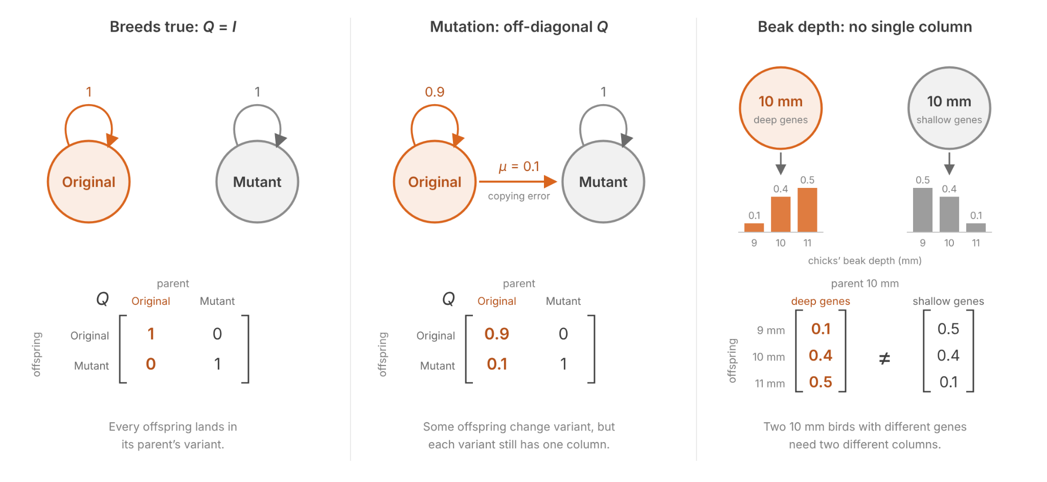
The replicator–mutator equation tracks a list of variants. Selection multiplies the count of each variant by its fitness through the fitness matrix W. Heredity (Q), the process by which offspring resemble their parents, moves offspring into variants:

$n^{\prime} = QWn$

A variant is a class of individuals that meets three requirements:

1. Same fitness: one entry of W per variant.
2. Same kinds of offspring: one column of Q per variant.
3. Breeds true: that column is the identity’s.

Mutation relaxes the third condition by letting Q be nonzero off the diagonal, hence its usual name, the mutation matrix. But finches grouped by beak depth break the second condition. Finches with the same beak depth don’t all produce the same kind of offspring. Two finches with 10 mm beaks can carry different genes, and so have different chicks.

But we can still reason about the average beak depth, and how it changes. Consider finches grouped by their beak depths. Let’s imagine a particular class i with beak depths between 10.0 and 10.1 mm. Then:

1. $xᵢ$ is the class frequency: the number of birds in the class, divided by the population size.
2. $wᵢ$ is its average number of offspring.
3. $zᵢ$ is its average beak depth (e.g., about 10.05 mm).
4. $\textstyle \varDelta z_i$ is the change from $zᵢ$ to their offspring’s average beak depth.

Next, count the offspring by their parent’s class, not their own. Let $xᵢ′$ be the fraction of chicks that descend from class i, and $zᵢ′$ the mean beak depth of those chicks. The change in mean beak depth is:

$\displaystyle \varDelta\bar{z} = \bar{z}^{\prime}-\bar{z} = \sum_i x_i^{\prime} z_i^{\prime}-\sum_i x_i z_i$

We also let $z̄*$ be the parents’ mean beak depth, with each parent counted once per chick:

$\bar{z}^{*} = \sum_i x_i^{\prime}\,z_i$

Mean fitness w̄ is the average number of offspring per parent, and wᵢ/w̄ is the class’s relative fitness. Then:

• $xᵢ′ = xᵢwᵢ/w̄$ multiplies class frequency by relative fitness.
• $\textstyle z_i^{\prime} = z_i + \varDelta z_i$ᵢ adds the chicks’ shift to their parents’ mean.

The change in mean beak depth can be expressed as two differences.

$\displaystyle \varDelta\bar{z} = (\bar{z}^{*}-\bar{z}) + (\bar{z}^{\prime}-\bar{z}^{*})$

In the first step, parent classes that leave more chicks pull the mean toward their beak depth. Appendix A shows that the shift is set by the covariance of fitness and trait:

$\bar{z}^{*}-\bar{z} = \frac{\operatorname{Cov}(w,z)}{\bar{w}}$

In the second step, the chicks of class i sit Δzᵢ from their parents’ mean. Averaged over all chicks, the second step is (Appendix A):

$\displaystyle \bar{z}^{\prime}-\bar{z}^{*} = \frac{\operatorname{E}(w \varDelta z)}{\bar{w}}$

Add the two steps. The result is the Price equation (Price 1970):

$\displaystyle \varDelta\bar{z} = \frac{\operatorname{Cov}(w,z)}{\bar{w}} + \frac{\operatorname{E}(w \varDelta z)}{\bar{w}}$

The Price equation has two terms:

1. The first term is the selection differential S: the change selection alone would make if every offspring were a copy of its parent. It comes from the first step, which for listed variants comes from the fitness matrix W.
2. The second term is the transmission T: how far offspring differ from their own parents, averaged over all offspring. It comes from the second step, which for listed variants comes from the mutation matrix Q. Other sources write T out in full; the letter is this post’s.
3. R, the response to selection, is another name for the left side, Δz̄. The name assumes that selection moved the mean, though T can move it with no selection at all, for example through mutation bias or a change in environment.

Another way to express the Price equation, then, is:

$R = S + T$

Classically, selection is split into three episodes: survival to breeding age, mating success, and fecundity (Arnold & Wade 1984). Our drought data cover only survival, so we assume that survival is all of selection. In other words, survivors of every beak depth raise the same number of chicks on average, a constant c:

$\operatorname{E}(\text{chicks} \mid \text{survived}, z) = c$

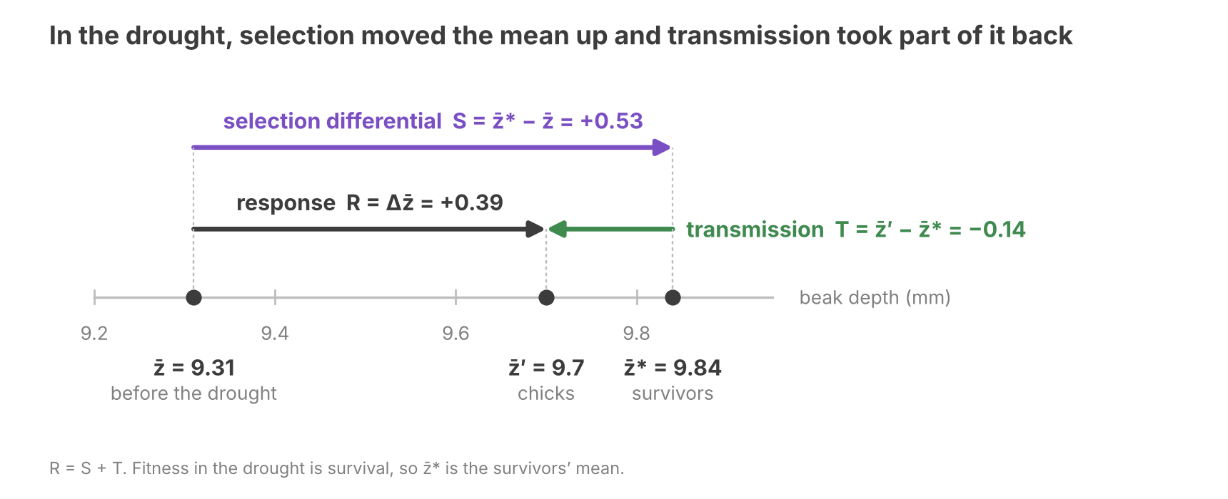
With this assumption, $xᵢ′$ is the fraction of survivors in class i. So $z̄*$, the mean after selection, is the survivors’ mean. The figure puts the drought’s means on a number line, using the chicks’ mean that a later section predicts:

The Price equation holds for any trait and any rule of inheritance. Changing bin size doesn’t change R, only the balance between S and T.

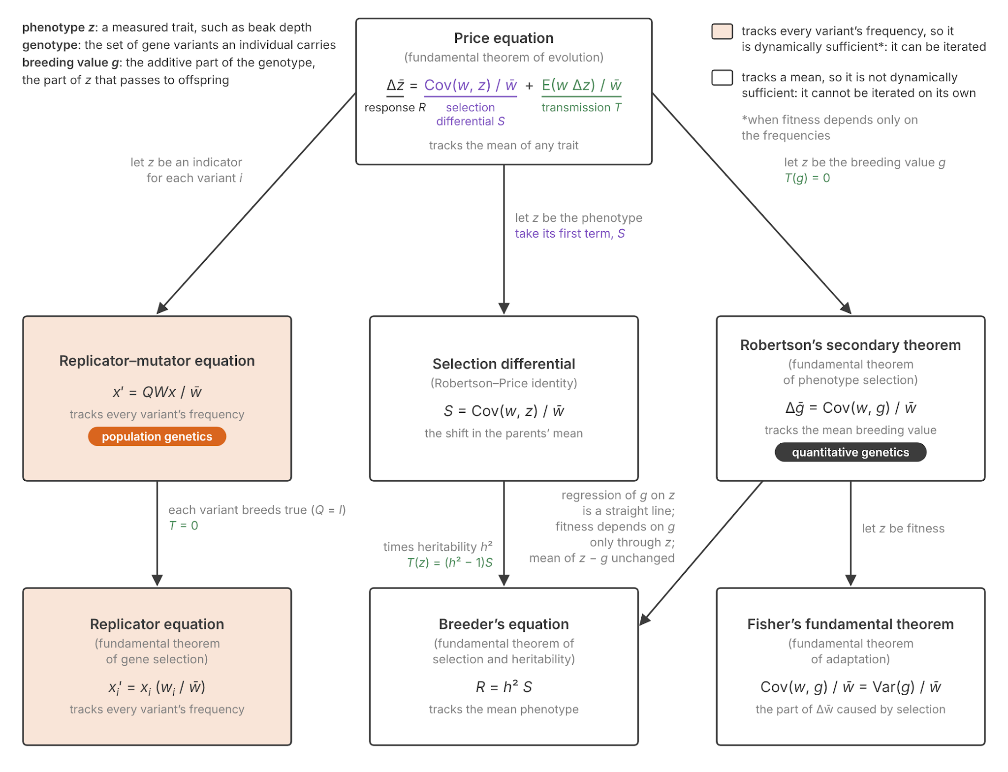
The Price equation is described by Queller (2017) as the fundamental theorem of evolution. It sits at the top of a family of classical results, bridging the gap between methods in population genetics and quantitative genetics. The following tree is adapted from his, and our section titles use his names.

The Theorem of Gene Selection

This section derives the replicator equation from the Price equation, following the left branch of the tree.

Let z be an indicator variable: 1 for variant i, and 0 for other variants. The mean of an indicator variable is its frequency:

$\bar{z} = x_i$

The left side of the Price equation becomes:

$\displaystyle \varDelta\bar{z} = \bar{z}^{\prime}-\bar{z} = x_i^{\prime}-x_i = \varDelta x_i$

Substitute the indicator into S. Only variant i has z = 1, so only its fitness enters the covariance (Appendix B):

$\frac{\operatorname{Cov}(w,z)}{\bar{w}} = x_i\,\frac{w_i-\bar{w}}{\bar{w}}$

This is the replicator equation’s change in frequency: what selection does when every offspring copies its parent.

An offspring of a variant-k parent lands in variant i with probability $\textstyle Q_{ik}$. That probability is the mean z of its offspring, so the change in z for a variant-k parent is:

$\displaystyle \varDelta z_k = Q_{ik}-z_k$

For variant i, T measures the balance of mutation inflow and outflow:

$\displaystyle \frac{\operatorname{E}(w \varDelta z)}{\bar{w}} = \text{inflow}-\text{outflow} = \frac{\sum_{k\neq i} Q_{ik} w_k x_k}{\bar{w}}-\frac{(1-Q_{ii}) w_i x_i}{\bar{w}}$

Add S and T to $xᵢ$. Every term cancels except the flow through Q (Appendix B):

$x_i^{\prime} = \frac{\sum_k Q_{ik}\,w_k\,x_k}{\bar{w}}$

In matrix form, with W the diagonal matrix of fitnesses, this is the replicator–mutator equation in frequencies:

$x^{\prime} = \frac{QWx}{\bar{w}}$

If each variant breeds true, Q is the identity matrix and T vanishes. The sum for $xᵢ′$ then keeps only its k = i term, which is the replicator equation:

$x_i^{\prime} = x_i\,(w_i/\bar{w})$

The three equations form a ladder, each rung more general than the one below:

• The replicator equation tracks the frequency of every variant and assumes each variant breeds true.
• The replicator–mutator equation also tracks every frequency, and lets copying errors move offspring between listed variants.
• The Price equation tracks the mean of any trait, and allows any rule of inheritance.

We now turn our attention to quantitative genetics. All of its equations require an extra assumption to predict past one generation. The Moment Hierarchy section explains why.

The Selection Differential

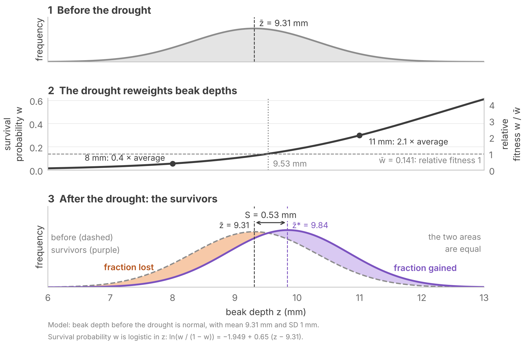
Let’s reconsider how drought affected beak depth:

Recall that the selection differential S is the shift in means before and after selection:

$S = \bar{z}^{*}-\bar{z}$

In the drought, the mean rose from 9.31 mm to 9.84 mm among the survivors (Grant 1986), so S is 0.53 mm.

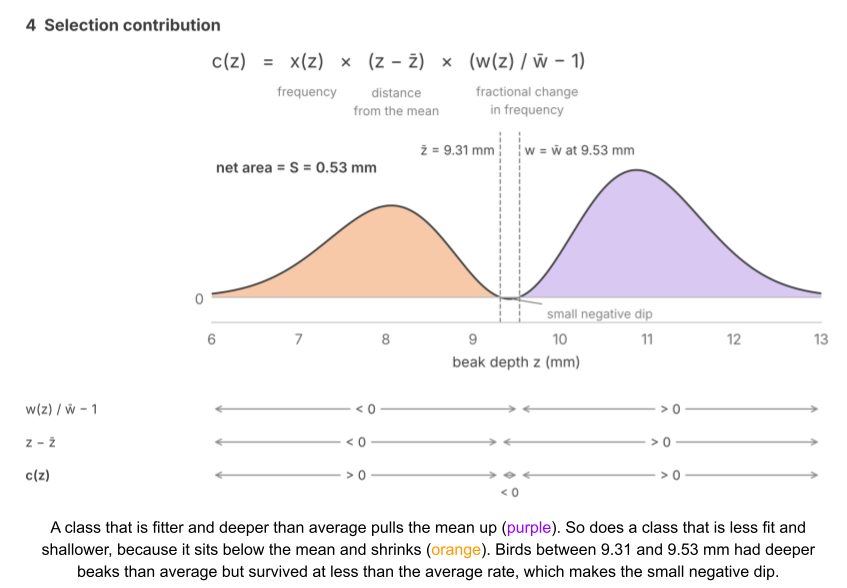
Written out, S sums the product of two deviations, weighted by class frequency xᵢ:

$\displaystyle S = \sum_i x_i\left(\frac{w_i}{\bar{w}}-1\right)(z_i-\bar{z}) = \frac{\operatorname{Cov}(w, z)}{\bar{w}}$

1. $wᵢ/w̄ − 1$ sets how much its fraction changed.
2. $zᵢ − z̄$ sets how far from the mean that fraction sits.

Covariance measures net alignment between these deviations. When matching signs dominate, selection raises the mean. When opposite signs dominate, selection lowers it.

Biologists measure S in the field the way the Grants did. They measure a trait across individuals, while also recording who survives or reproduces. Over 2,500 estimates of selection from 63 studies show that most selection in nature is weaker than in the drought (Kingsolver et al 2001). Breeders instead impose S, by choosing which animals breed.

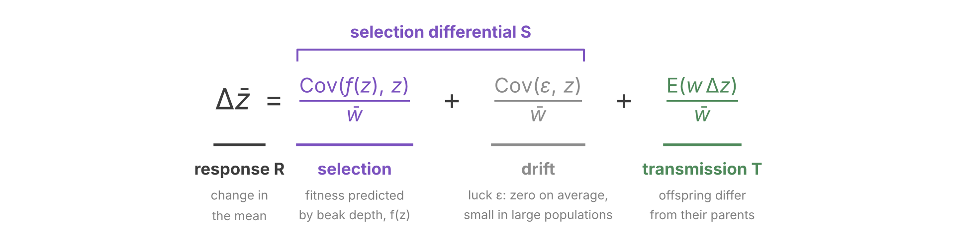
S mixes two causes of differential reproduction: trait and luck. To separate them, imagine replaying the drought many times with the same birds. Let expected fitness $f(z)$ be the average fitness of birds with beak depth z over the replays. A bird’s fitness w is what it actually had in this one drought. It differs from expected fitness by ε, the part of its fitness that beak depth does not explain:

$w = f(z) + \varepsilon$

Averaged over the replays, ε is zero at every beak depth:

$\operatorname{E}(\varepsilon \mid z) = 0$

So ε has no covariance with beak depth on average, but in any one drought luck makes it covary by chance. Taken together, we have decomposed S into two terms.

The rest of this post will assume a large population, where drift is small.

The Breeding Value

S is a shift in the parents, and the population evolves only if the offspring shift too. But heredity passes on genes, not beak depth. A bird’s beak depth also depends on its conditions as a chick, such as the food it received, and that part usually doesn’t pass on. So the offspring keep only part of S. To find how S is carried across generations, we need to decompose z.

A phenotype (z) is a measured trait, such as beak depth. An individual’s breeding value (g) is the part of its phenotype that its offspring inherit on average. Call the rest u:

$z = g + u$

What g contains depends on how the species reproduces. A genotype is the set of gene variants an individual carries, and its genotypic value (G) is the average phenotype of individuals that carry it.

In clonal reproduction, the whole genotype passes intact to the offspring, so the breeding value is the genotypic value and the rest is environmental deviation (e):

$g = G, \quad u = e$

But in sexual reproduction only part of G passes. A parent passes along only one allele per locus.

Imagine a locus with two equally prevalent alleles B and b. BB, Bb and bb birds have beaks 9.4, 9.4 and 9.0 mm deep, respectively. With random mating, Bb birds are twice as common as BB or bb birds, so the population mean is:

$\bar{z} = \tfrac{1}{4}(9.4) + \tfrac{1}{2}(9.4) + \tfrac{1}{4}(9.0) = 9.3\text{ mm}$

A chick gets one allele from each parent, so its second allele is B or b with equal odds. Chicks that get B average 9.4 mm whatever their second allele, and chicks that get b average 9.2 mm, halfway between 9.4 and 9.0. Measured from 9.3, that is +0.1 and −0.1 mm. Adding a bird’s two allele effects to the population mean gives its breeding value. And indeed, offspring of a Bb finch average 9.3 mm, not 9.4 mm. Dominance (D) is the remainder: genotypic value minus breeding value. It denotes the interaction between the two alleles at one locus.

Genotype	Genotypic value (G)	Breeding value (g)	Dominance (D)
bb	9.0 mm	9.1 mm	−0.1 mm
Bb	9.4 mm	9.3 mm	+0.1 mm
BB	9.4 mm	9.5 mm	−0.1 mm

Interactions between alleles at different loci, epistasis (I), are mostly broken up the same way when meiosis reshuffles alleles across loci.

In a sexual species, then, the genotypic value has three parts:

$G = g + D + I$

Substitute it into the phenotype:

$z = (g + D + I) + e$

With minor exceptions, a parent passes on its g but not its D or I, so for transmission D and I behave like e. So the rest u holds all three:

$u = D + I + e$

The Theorem of Phenotype Selection

Recall that beak depth splits into its breeding value g and the rest u:

$z = g + u$

To apply the Price equation to all three variables, we write the trait as an argument. For any trait y:

$R(y) = S(y) + T(y)$

$\displaystyle S(y) = \frac{\operatorname{Cov}(w,y)}{\bar{w}}, \quad T(y) = \frac{\operatorname{E}(w \varDelta y)}{\bar{w}}, \quad R(y) = \varDelta\bar{y}$

Without an argument, S, T and R refer to z.

We begin with one assumption, faithful transmission: the chicks’ mean g equals the mean g of their parents, so T(g) vanishes. In a sexual species, faithful transmission also requires fair meiosis: each allele must have an equal chance of reaching a chick. Mutation and meiotic drive break these assumptions, respectively.

$\displaystyle T(g) = \frac{\operatorname{E}(w \varDelta g)}{\bar{w}} = 0$

Apply the Price equation to g. Faithful transmission removes T(g):

$\Delta\bar{g} = \frac{\operatorname{Cov}(w,g)}{\bar{w}}$

That is:

$R(g) = S(g)$

This is Robertson’s secondary theorem of natural selection (Robertson 1966; Price 1970). Like the Price equation, this theorem generalizes to any heritable state, not just nucleic acids. It applies for any state that offspring receive faithfully, such as the song a male finch learns from its father (Grant & Grant 1996).

But g is a latent variable. To model how observable z changes, we need a second assumption. We assume parents only pass down g, and nothing else that shapes the trait, and that the environment stays the same. Then each chick draws a fresh e, and meiosis gives it fresh D and I. Then R(u) vanishes.

$\displaystyle R(u) = \varDelta\bar{u} = 0$

Applying Price on u:

$0 = S(u) + T(u)$

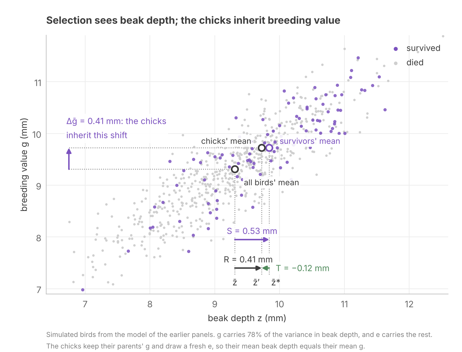
Selection sorts the finches by z, but the chicks inherit g. Some survivors had deep beaks due to environmental factors, so the survivors’ mean g moved less.

Splitting z splits the covariance:

$\operatorname{Cov}(w,z) = \operatorname{Cov}(w,g) + \operatorname{Cov}(w,u)$

Divide both sides by w̄:

$S(z) = S(g) + S(u)$

S(g) is the shift the chicks inherit, and the environmental covariance S(u) is the part they do not. Note that u can hold dominance and epistasis, which are genetic but are broken up by meiosis.

On the Isle of Rum, red deer with heavier antlers have more offspring. Yet over nearly 30 years, the average antler size did not increase, despite the trait being heritable (Kruuk et al 2002). The authors proposed a nutrition confound: a well-fed stag grows heavy antlers and also wins more contests for mates. Nutrition contributes to S(u), which explains nearly all of S.

We have applied the Price equation to three variables. We can visualize this as a table, and our assumptions correspond to zeroed cells. Every other cell follows.

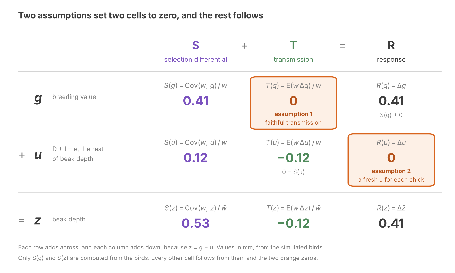
The rest of this post builds on Robertson’s theorem. Breeding values cannot be observed directly, so The Breeder’s Equation estimates this covariance from traits we can measure. Fisher’s fundamental theorem takes fitness itself as the trait.

The Breeder’s Equation

Heredity carries g, so a phenotype is a noisy measurement of the part that passes on. The results of The Reliability Ratio carry over directly:

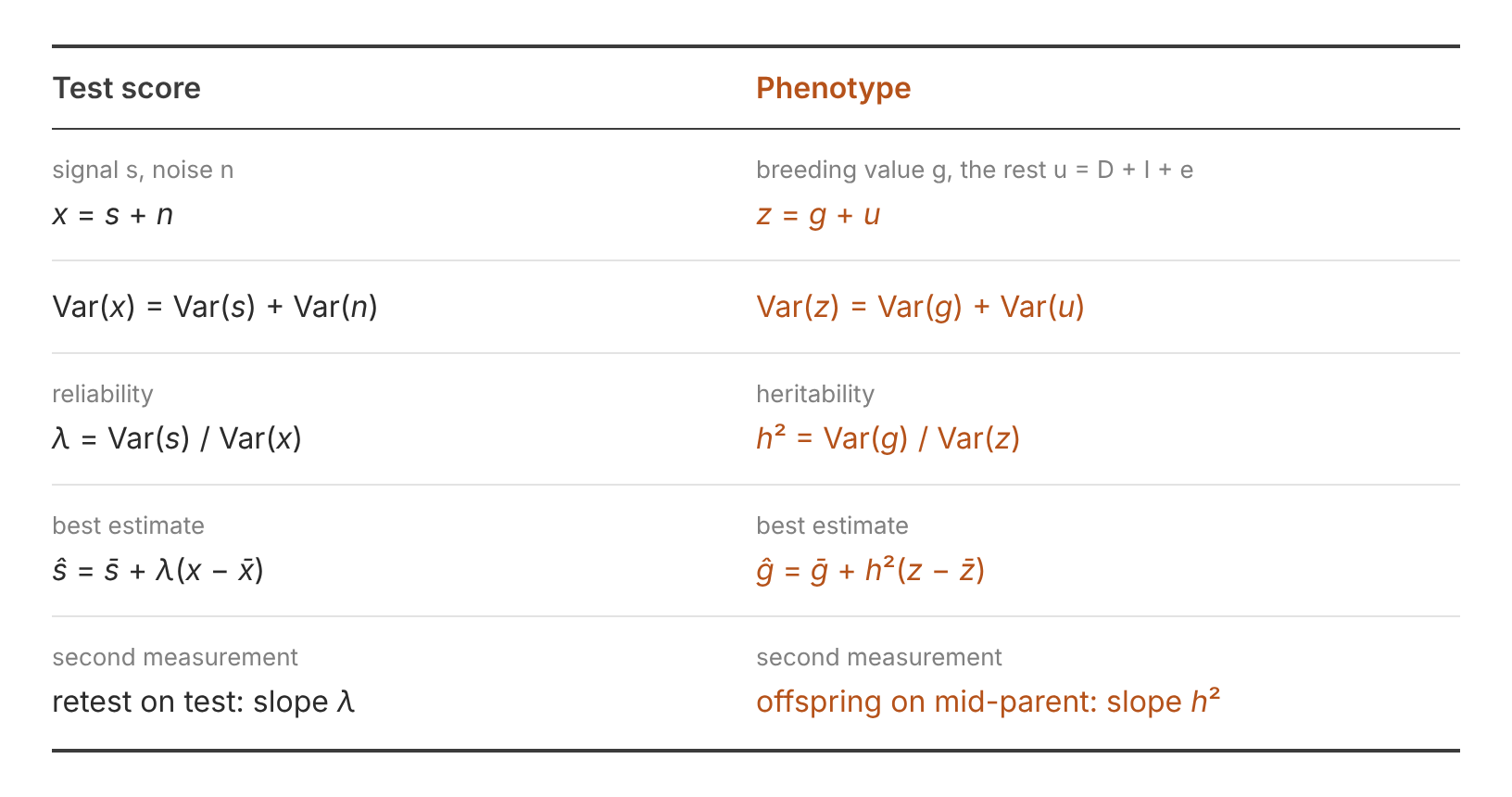
The estimate starts from a regression. When u is independent of g, the slope of the regression g on z is the reliability:

$\frac{\operatorname{Cov}(g,z)}{\operatorname{Var}(z)} = \frac{\operatorname{Var}(g)}{\operatorname{Var}(z)} = h^2$

Here, we call the reliability the narrow-sense heritability (h²), the fraction of the variance in beak depth that comes from breeding values.

To derive the breeder’s equation, we need Kelley’s rule from The Reliability Ratio. That requires two assumptions. First, u is independent of g, as the slope above assumed. Second, g and u are normally distributed. Kelley’s rule then puts the average g at each beak depth on the regression line:

$\operatorname{E}(g \mid z) = \bar{g} + h^2\,(z-\bar{z})$

Here we need one more assumption: fitness depends on g only through z.

$\operatorname{E}(w \mid z, g) = \operatorname{E}(w \mid z)$

Fitness sees only z, so it sees g only through the average g at each beak depth, and Kelley’s rule shrinks that average toward the mean by h². Appendix C works through the steps. The result converts Robertson’s covariance into one we can measure:

$\operatorname{Cov}(w,g) = h^2\,\operatorname{Cov}(w,z)$

Divide both sides by w̄, and apply Robertson’s theorem:

$R(g) = S(g) = h^2 S$

Recall that $z = g + u$. This splits the response to selection:

$R = R(g) + R(u) = h^2 S + R(u)$

The second assumption of The Theorem of Phenotype Selection removes the last term:

$R = h^2 S$

This is the breeder’s equation. It splits Robertson’s covariance into two factors, S for selection and h² for the fraction of S that passes on, so that each can be measured on its own.

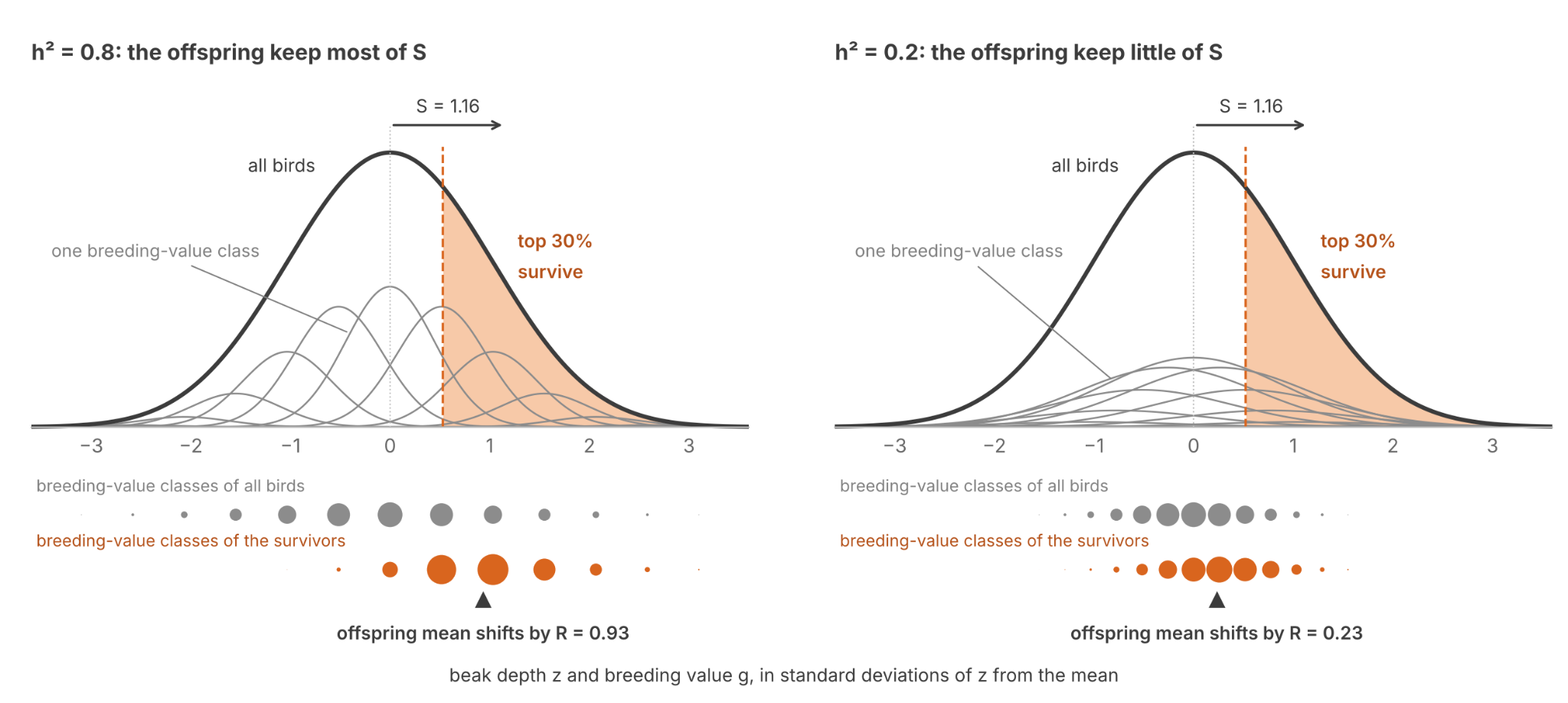
The figure shows how heritability sets the response. Each gray curve is one breeding-value class, and the black curve is the whole population, with beak depth in standard deviations. Both panels have the same population curve, and the same selection pressures, so S is the same. The survivors differ. On the left, the classes are narrow, and the survivors come mostly from classes far to the right. On the right, the classes are wide, and the survivors come mostly from classes near the middle. The offspring inherit their parents’ breeding values, so R is 0.93 SD on the left and 0.23 SD on the right.

For the finches, Boag (1983) measured a heritability of 0.78 for beak depth. The breeder’s equation predicts the response in the offspring of the survivors:

$R = 0.78\times 0.53\text{ mm} = 0.41\text{ mm}$

That predicts a mean of 9.72 mm for the chicks.

Recall that T = R − S. Now, substitute the breeder’s equation and factor:

$T = h^2 S-S = (h^2-1)\,S$

For beak depth:

$T = (0.78-1)\times 0.53\text{ mm} \approx -0.12\text{ mm}$

$0.41 \approx 0.53 + (-0.12)$

The 0.12 mm that does not pass on is T for beak depth. The breeder’s equation predicts that the chicks of deep-beaked survivors fall back toward the mean. This is regression to the mean. Tracked through g instead, the whole response is S(g) and T(g) vanishes.

Heredity, heritability and transmission are easy to conflate.

• Heredity (Q) is an individual process across generations. It denotes what each child inherits from its parents.
• Heritability (h²) is a population statistic within a generation. It denotes what fraction of trait variance comes from the breeding value. It describes how individuals differ.
• Transmission (T) is a population statistic across generations. It denotes change in the mean between selected parents and their offspring. It collects mutation, and everything else that separates children from their parents. Only on the breeder’s assumptions does h² fix T for a given S.

Neither h² nor S alone produces R. If h² = 0, selection acts on the parents but cannot affect the children. If S = 0, heritable state can be copied faithfully, yet selection does not move the mean. Schulman et al (2012) built DNA tiles with high copying fidelity, but every pattern grew at the same rate.

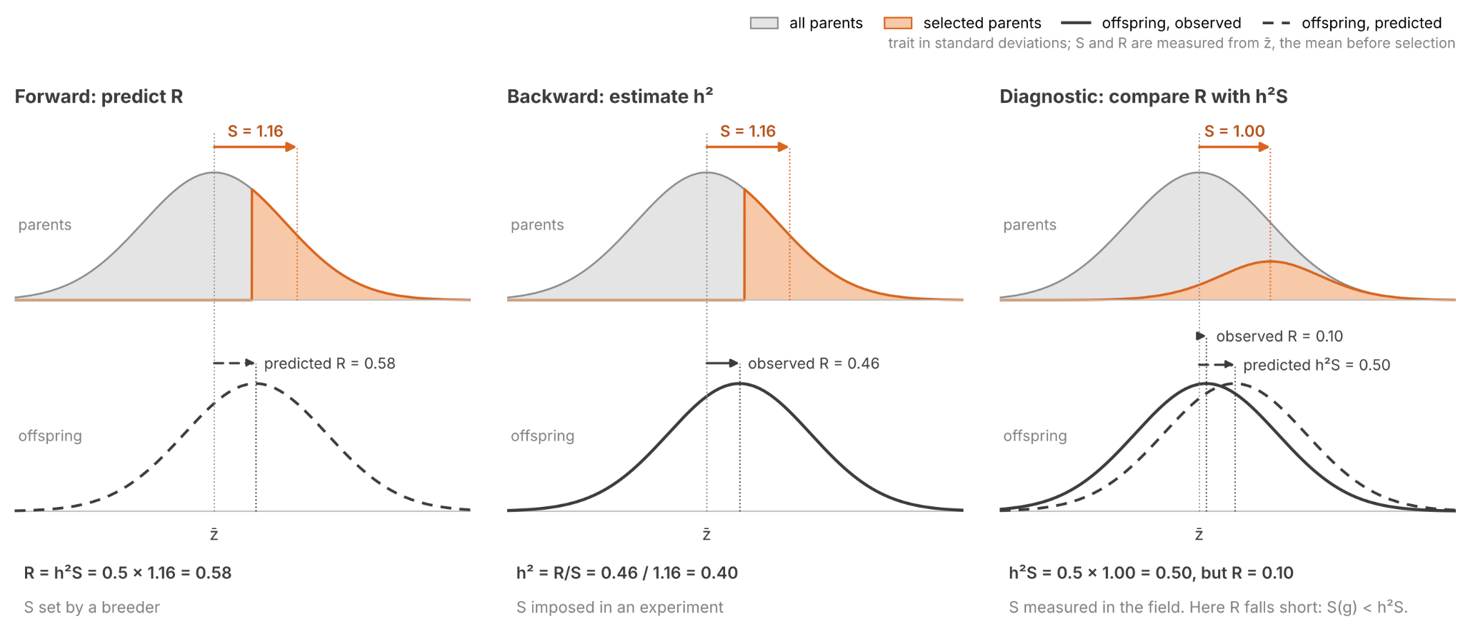
The breeder’s equation can be applied in three ways: forward, backward and diagnostic.

First, if h² and S are known, breeders can forecast R. They use this method to plan their selection process. Conservation biologists calculate whether a population will keep pace with a changing environment.

Second, a selection experiment controls the value of S and measures the resultant response R. Heritability is learned by taking their ratio.

Third, biologists can predict R from the model, and then compare it with the observed R. Prediction errors suggest an assumption mismatch. Here are two cases which challenge the assumption that fitness depends on g only through z.

• Heritable traits under strong directional selection often change less than predicted (Merilä et al 2001). The red deer on Rum are one such case. Nutrition drives both antler size and fitness. When fitness depends on the environment directly, S(g) is smaller than the breeder’s equation predicts. In other words, S(g) < h²S.
• Grant & Grant (1995) measured both drought generations. Mean beak depth rose from 9.21 mm before the drought to 9.70 mm in the chicks hatched in 1978. In contrast with the breeder’s prediction, the chicks kept nearly all of the survivors’ shift. Why? Well, the drought also favored larger bodies, and birds that inherit larger bodies tend to inherit deeper beaks. When selection also acts on a second trait whose breeding value covaries with g, S(g) can exceed the prediction. In other words, S(g) > h²S.

The forward and diagnostic uses require knowing h². How do we measure it?

Galton (1886) invented regression to study heredity. Plot each offspring’s trait against the average of its parents, the mid-parent, and fit a line. If offspring were identical to their parents, the line would have slope 1. If chicks inherited nothing from their parents, the slope would be 0. For finch beak depth, the slope is 0.78.

Regression to the mean occurs because offspring play the role of the retest. On average, a chick inherits the g of its mid-parent, but it draws a fresh u. So the slope is the heritability h² (i.e., reliability).

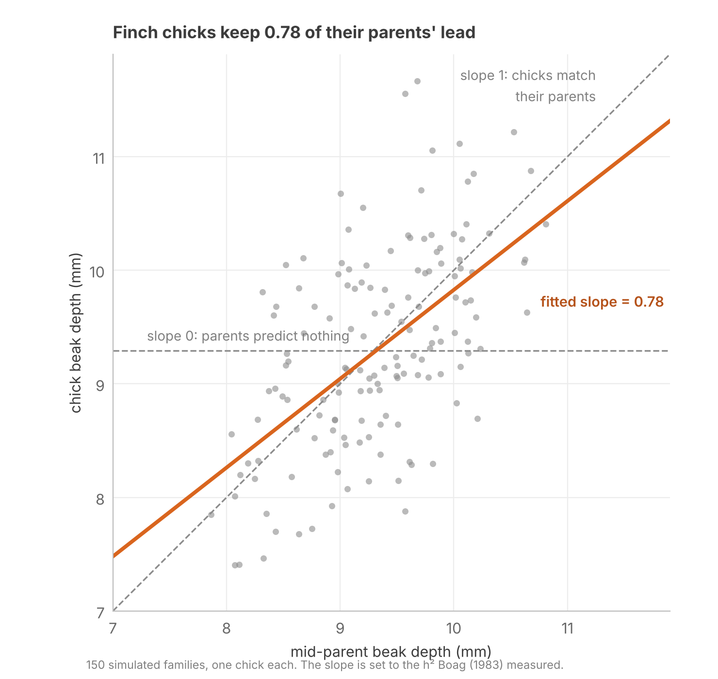
This conclusion only holds when its assumptions are met. The second assumption of The Theorem of Phenotype Selection fails if parents pass along non-genetic components (e.g., territory). In that situation, the slope measures breeding values and inherited environment together.

Fisher’s Fundamental Theorem

Selection improves organisms. Fisher sought to quantify the speed of improvement. He compared his result to the second law of thermodynamics: each law names a quantity that moves only one way.

Choose fitness itself as the trait. Setting z = w in the Price equation gives

$\displaystyle \varDelta\bar{w} = \frac{\operatorname{Var}(w)}{\bar{w}} + \frac{\operatorname{E}(w \varDelta w)}{\bar{w}}$

$R(w) = S(w) + T(w)$

Split fitness like any other trait: w = g + u. Recall the definition of S(g), but substitute g+u into the covariance:

$S(g) = \frac{\operatorname{Cov}(w,g)}{\bar{w}} = \frac{\operatorname{Cov}(g+u,\,g)}{\bar{w}}$

The covariance splits in two, and the covariance of g with itself is its variance. u is uncorrelated with g, so the last term is zero:

$S(g) = \frac{\operatorname{Cov}(g,g) + \operatorname{Cov}(u,\,g)}{\bar{w}} = \frac{\operatorname{Var}(g) + 0}{\bar{w}}$

Applying Robertson’s secondary theorem yields the change in mean fitness caused by selection:

$R(g) = S(g) = \frac{\operatorname{Var}(g)}{\bar{w}}$

This is Fisher’s (1930) fundamental theorem of natural selection. The rate of increase of fitness depends on Var(g), known as the additive genetic variance.

Dividing by w̄ once more gives the fraction by which selection raises mean fitness each generation: $Var(g)/w̄²$. Houle (1992) called this measure evolvability, a scale on which traits and species can be compared.

Only 15% of the finches on Daphne Major survived the 1977 drought, so the variance in relative fitness was enormous:

$\operatorname{Var}(w)/\bar{w}^{2} = 0.85/0.15 \approx 5.7$

But only its heritable part, Var(g), moved the next generation. If survival had been truly random, the population would not have changed.

Selection runs on heritable variance in fitness. If you measure it, you can predict how quickly selection will proceed. Recall that selection also uses up its fuel. An allele that raises fitness approaches fixation, and a fixed allele adds nothing to Var(g).

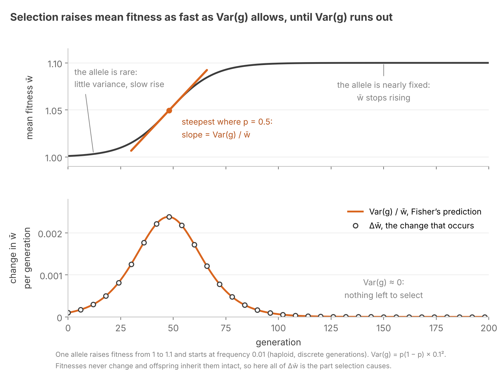
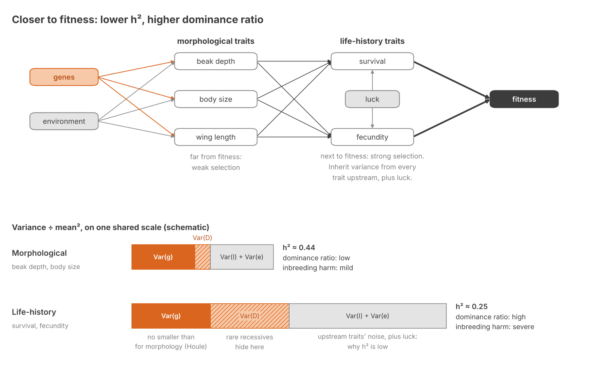
Selection tends to drain Var(g) faster than Var(D). Let’s name the dominance ratio:

$\text{dominance ratio} = \frac{\operatorname{Var}(D)}{\operatorname{Var}(g)}$

Harmful recessive alleles increase the dominance ratio. In heterozygotes they are masked by dominant alleles. Selection sees them only in the rare homozygotes, so they linger, and most of the variance they cause is Var(D). Inbreeding exposes these hidden recessives by making them homozygous.

The more fitness-relevant the trait, the higher its dominance ratio tends to be. Life-history (LH) traits such as survival, fecundity and development time are very correlated with fitness. They mediate much of the fitness impact of morphological traits. And indeed, in wild species LH traits have higher dominance ratios (Crnokrak & Roff 1995). In sand crickets, inbreeding harms LH traits far more than it harms body size (Roff 1998). LH traits also have lower heritabilities (Mousseau & Roff 1987), mostly because Var(u) is greater (Houle 1992).

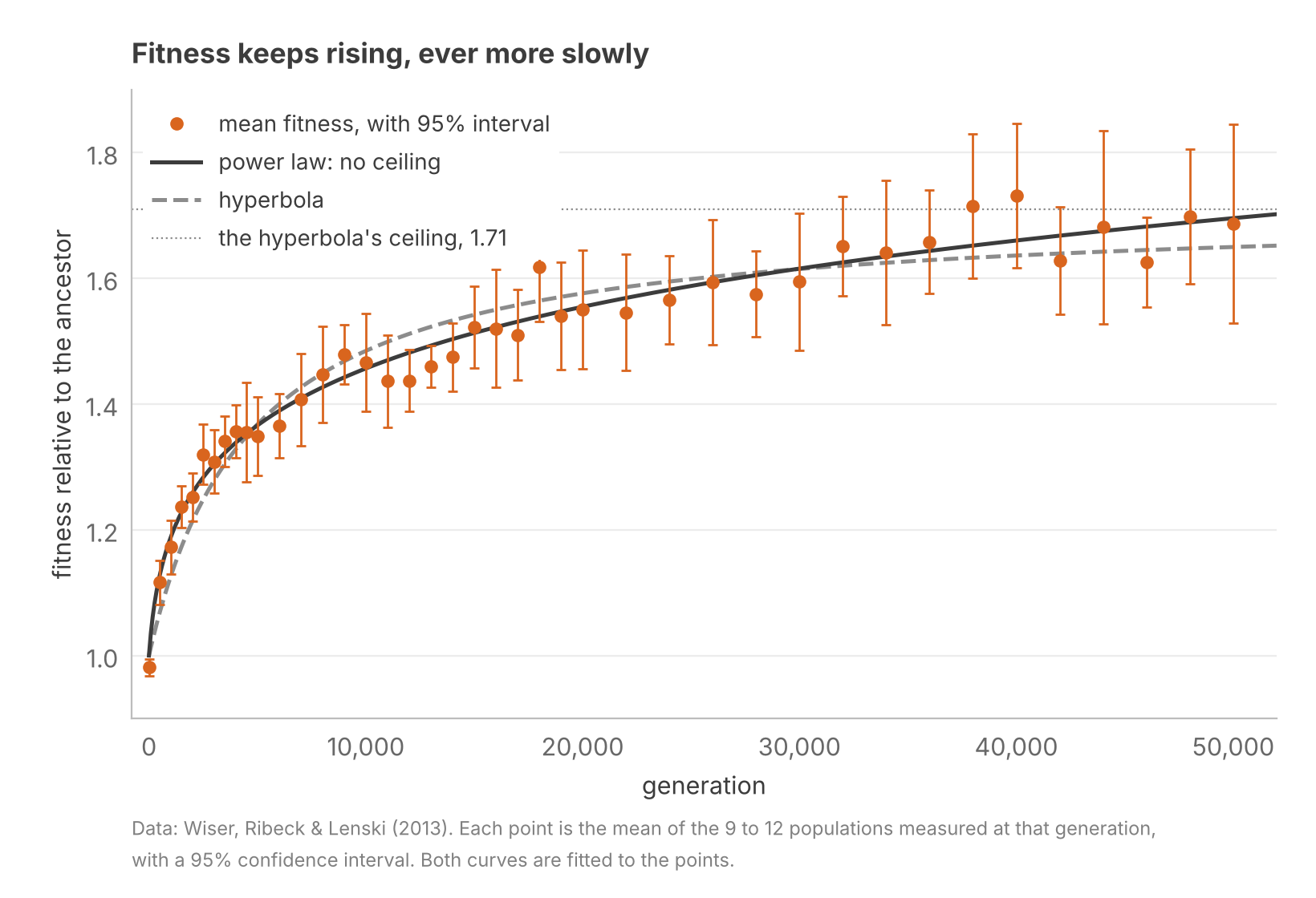
Does selection eventually stall? Mutation resupplies Var(g). But most mutations are harmful, so it also lowers fitness. In the replicator–mutator equation, the two settle into a balance where mean fitness stops rising. Do real populations reach that balance?

Lenski’s long-term evolution experiment (LTEE) addresses this question. Twelve populations of E. coli have grown in the same glucose-limited medium since 1988. Their fitness rose for 50,000 generations. The data fit a model with no ceiling better than one with a ceiling (Wiser et al 2013). The balance has not yet been reached.

The balance arrives when almost every new mutation is harmful. But a bacterial genome offers a very large search space. The topography of fitness landscapes is such that each selective sweep adds less fitness than the last, but they keep coming (Khan et al 2011).

Lenski’s medium never changes. But in the wild, the world changes too. The theorem does not guarantee an increase in mean fitness. Price (1972) and Frank & Slatkin (1992) showed that Fisher meant only the part of the change that selection causes. Fitness splits into g and u, so its change does too:

R(w) = R(g) + R(u)

For fitness, the assumption that R(u) = 0 breaks down. Offspring inherit their parents’ breeding value for fitness, but not their parents’ world. The climate may change. Rival species may evolve. And fitness can vary with intrapopulation changes, such as density or changes in variant frequencies. Fisher called all of these cases of nonzero R(u) the deterioration of the environment. A population can gain fitness through selection every generation while its mean fitness stays flat.

The Moment Hierarchy

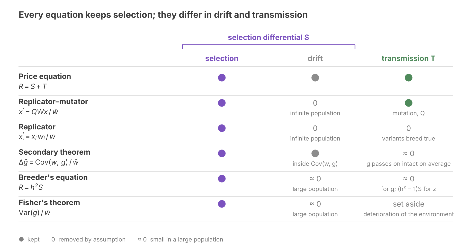
We have finished our survey of models derived from Price. They come in three categories.

• Identity models predict nothing. They model a change that has already happened.
• One-step models require data on the present population plus rules for fitness and transmission. Their assumptions permit prediction across one generation.
• Closed model predictions can be used as new data, which allow for repeat predictions. They allow forecasting change across time.

Why do some of our models reach the third level, while the rest stop at the second? The answer lies in which summaries of the population each model tracks, and whether those summaries predict their own future.

The mean is the first moment of the trait’s distribution: the average of z itself. The kth moment, for k above 1, averages the kth power of each individual’s deviation from the mean:

$\displaystyle \operatorname{E}((z-\bar{z})^k)$

The second moment is the variance. Squaring makes every deviation positive, so it measures spread. The third moment measures skew.

The Price equation updates the first moment, in our case the change in mean beak depth. But two finch populations with the same mean can have dramatically different means after one generation. Consider a population of finches with three variants, each with a distinct beak depth:

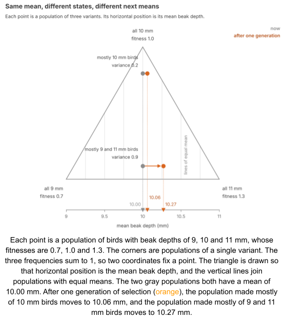
Lewontin (1974) called a set of variables dynamically sufficient when it predicts its own future. With three variants, the mean is not dynamically sufficient. Knowing the mean is not enough to predict how it will change.

To see why, let’s regress w on z. The covariance in S is the slope β of this regression multiplied by the variance:

$S = \frac{\operatorname{Cov}(w,z)}{\bar{w}} = \frac{\beta\,\operatorname{Var}(z)}{\bar{w}}$

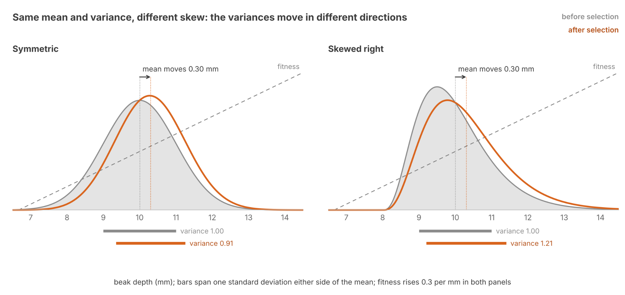
So the change in mean depends on variance. And the change in variance under selection depends on skew. Write $Var*(z)$ for the variance after selection. If fitness is a straight line in the trait:

$\displaystyle \operatorname{Var}^{*}(z)-\operatorname{Var}(z) = \frac{\beta \operatorname{E}((z-\bar{z})^3)}{\bar{w}}-S^2$

So two populations with the same first and second moments can still change differently, if their third moments differ.

The pattern continues up the chain. The change in each moment depends on the next higher moment. This chain of dependencies is the moment hierarchy. In general, no finite set of moments predicts its own future.

There are two ways to cut the chain and accomplish moment closure, one for discrete traits and one for continuous traits.

Discrete closure is exact. Recall the three-variant triangle above. Switching to two variants, the triangle shrinks to a line segment. If the two variants have beak depths $z₁$ and $z₂$, and the first has frequency x, the mean is:

$\bar{z} = x\,z_1 + (1-x)\,z_2$

Solve for x. Since z₁ and z₂ are fixed, the frequency follows from the mean alone (as long as the denominator is nonzero).

$x = \frac{\bar{z}-z_2}{z_1-z_2}$

So the variance is also a function of the mean alone:

$\operatorname{Var}(z) = x(1-x)(z_1-z_2)^2 = (\bar{z}-z_2)(z_1-\bar{z})$

We saw that S needs the variance. But the variance only needs the mean. The chain closed after the first moment.

But as the triangle showed, with three variants the mean is not dynamically sufficient. In such cases, we can achieve closure by instead using indicator variables for each variant. Their means are the variant frequencies, and together the frequencies fix the population. Writing the Price equation once per indicator gives the replicator–mutator equation.

We defined a variant as having members with the same fitness and the same kinds of offspring. So for each variant, W and Q are fixed tables, or depend only on the frequencies, and w̄ is determined from variant frequencies. The equation updates frequencies, and can be iterated to forecast into future generations. Population genetics models are closed models.

Continuous closure is approximate. Without a finite list of variants, the chain must be cut by assumptions. The usual ones are that the trait stays normal and its variance stays steady. A normal distribution is fixed by its mean and variance. If the assumptions hold, dynamic sufficiency is obtained.

$R = h²S$ gives the response for one generation. To predict the next, the breeder’s equation assumes that h² and the variance of the trait stay the same. Selection changes both. Holding h² and the variance fixed cuts the chain, so the mean can predict its own future.

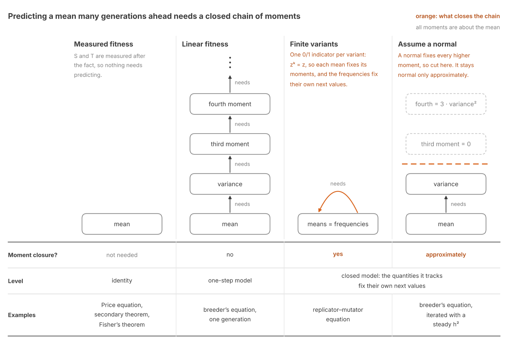
Continuous closure requires assumptions. What reason do we have to believe they are valid? Fisher (1918) answered with the infinitesimal model: a trait is the sum of the small effects of a large number of genes. Discrete closure is impractical here. A gene’s fitness depends on the genes it is paired with, so it would need one indicator per combination of genes, and there are astronomically many. However, by the central limit theorem, such a sum is close to normal. And because each gene’s effect is small, selection barely changes any gene’s frequency, so after an initial drop the variance holds steady. So the infinitesimal model generates conditions which make continuous closure’s assumptions approximately true.

The infinitesimal model is supported by modern genomic data. Genes of large effect do exist. In medium ground finches, one gene, HMGA2, has a large effect on beak size, and selection on it was strong during a later drought (Lamichhaney et al 2016). But genome-wide association studies (GWAS), which scan the whole genome for variants associated with a trait, have revealed that most complex traits are highly polygenic. For example, more than ten thousand variants together explain about 40% of the variance in height among people of European ancestry (Yengo et al 2022).

Applications

Our discussion so far has been fairly theoretical. Let’s close with some practical use cases.

First, let’s consider fisheries-induced evolution. Historically, fisheries usually bring the largest fish to market. This has the unfortunate side effect of leaving smaller fish to breed: selection for small body size. Since body size is heritable, the breeder’s equation predicts smaller fish in the next generation. Conover & Munch (2002) confirmed this in captive Atlantic silversides. The breeder’s equation also points to the remedy. Managers cannot change h², but they choose S. Catching fish at random brings S to zero, and purposefully releasing the largest fish makes it positive.

Second, animal breeders historically selected on the basis of traits like milk yield. But genomic selection estimates an animal’s g from its DNA at birth (Meuwissen et al 2001). By using information from the genotype instead of the phenotype, breeders can choose parents years earlier. Generations got shorter, and yearly gains rose by 50–100% for yield traits. Gains were especially pronounced for low heritability traits, where an animal’s own phenotype reveals little about its g (García-Ruiz et al 2016).

These theorems of evolution apply in situations not involving nucleic acids. Price (1995) called for a universal selection theory that would treat chemical, cultural and genetic selection alike, the way communication theory treats every kind of signal.

Does an economy grow because firms improve their own productivity, or because they outcompete other firms? Economists answer with the Price equation. Treat each firm’s productivity as the trait z, and its share of the industry’s output as its frequency x. Then S is reallocation: output shifting from unproductive to productive firms. T is self-improvement. Since a new firm has no parent, firm entry needs a term of its own. Firm turnover (entry and exit) shows up in both S and the entry term.

The answer depends on the industry. In 1980s US manufacturing, about 80% of productivity growth was T (Foster et al 2001). In 1990s US retail, virtually all labor productivity growth came from turnover: new stores replacing less productive ones (Foster et al 2006).

In industries where growth depends on turnover, keeping weak firms alive is costly. In 1990s Japan, banks kept lending to failing “zombie” firms. Industries full of zombies had lower productivity, and fewer healthy firms entered (Caballero et al 2008). In Price’s terms, without the loans the fitness of zombie firms would have been zero.

The contrast with biology is in transmission T. For beak depth, T is regression to the mean. Chicks inherit only the fraction h² of their parents’ advantage. So S does the work, and T gives part of it back. But for firms, T can be positive and drive most of an industry’s growth. T averages each firm’s change in productivity from its earlier self. While mutation is blind, firms change on purpose. Change that is aimed at improvement and then passed on is called guided variation (Boyd & Richerson 1985). Guided variation can make T positive without any selection: firms improve even if their shares never change.

Wrapping Up

We learned the following today.

1. The Price equation splits a response R of a variable into the selection differential S and transmission T. It holds for any trait and any rule of inheritance. It is an identity. But with rules for fitness and transmission, it can become a predictive model.
2. With an indicator for each variant, the Price equation becomes the replicator–mutator equation.
3. Tracking the breeding value g instead of the phenotype z removes T, leaving only S. This is Robertson’s secondary theorem.
4. The breeder’s equation says that only the fraction h² of S reaches the offspring.
5. Applied to fitness, the Price equation becomes Fisher’s fundamental theorem. Variance in heritable fitness is the fuel of selection.
6. Predicting many generations needs a closed model. Discrete traits can afford exact moment closure. Continuous traits can be closed approximately, through the infinitesimal model.

Until next time.

References

1. Arnold & Wade (1984). On the measurement of natural and sexual selection: theory.
2. Boag (1983). The heritability of external morphology in Darwin’s ground finches (Geospiza) on Isla Daphne Major, Galápagos.
3. Boyd & Richerson (1985). Culture and the evolutionary process.
4. Caballero et al (2008). Zombie lending and depressed restructuring in Japan.
5. Conover & Munch (2002). Sustaining fisheries yields over evolutionary time scales.
6. Crnokrak & Roff (1995). Dominance variance: associations with selection and fitness.
7. Fisher (1918). The correlation between relatives on the supposition of Mendelian inheritance.
8. Fisher (1930). The Genetical Theory of Natural Selection.
9. Foster et al (2001). Aggregate productivity growth: lessons from microeconomic evidence.
10. Foster et al (2006). Market selection, reallocation, and restructuring in the U.S. retail trade sector in the 1990s.
11. Frank & Slatkin (1992). Fisher’s fundamental theorem of natural selection.
12. Galton (1886). Regression towards mediocrity in hereditary stature.
13. García-Ruiz et al (2016). Changes in genetic selection differentials and generation intervals in US Holstein dairy cattle as a result of genomic selection.
14. Grant (1986). Ecology and Evolution of Darwin’s Finches.
15. Grant & Grant (1995). Predicting microevolutionary responses to directional selection on heritable variation.
16. Grant & Grant (1996). Cultural inheritance of song and its role in the evolution of Darwin’s finches.
17. Houle (1992). Comparing evolvability and variability of quantitative traits.
18. Khan et al (2011). Negative epistasis between beneficial mutations in an evolving bacterial population.
19. Kingsolver et al (2001). The strength of phenotypic selection in natural populations.
20. Kruuk et al (2002). Antler size in red deer: heritability and selection but no evolution.
21. Lamichhaney et al (2016). A beak size locus in Darwin’s finches facilitated character displacement during a drought.
22. Lewontin (1974). The Genetic Basis of Evolutionary Change.
23. Merilä et al (2001). Explaining stasis: microevolutionary studies in natural populations.
24. Meuwissen et al (2001). Prediction of total genetic value using genome-wide dense marker maps.
25. Mousseau & Roff (1987). Natural selection and the heritability of fitness components.
26. Price (1970). Selection and covariance.
27. Price (1972). Fisher’s “fundamental theorem” made clear.
28. Price (1995). The nature of selection.
29. Queller (2017). Fundamental theorems of evolution.
30. Robertson (1966). A mathematical model of the culling process in dairy cattle.
31. Roff (1998). Effects of inbreeding on morphological and life history traits of the sand cricket, Gryllus firmus.
32. Schulman et al (2012). Robust self-replication of combinatorial information via crystal growth and scission.
33. Wiser et al (2013). Long-term dynamics of adaptation in asexual populations.
34. Yengo et al (2022). A saturated map of common genetic variants associated with human height.

Appendix A: Deriving the Price Equation

This appendix derives the two steps of The Fundamental Theorem of Evolution. It uses the rules for counting chicks by their parent’s class, and the parents’ mean counted once per chick:

$\displaystyle x_i^{\prime} = \frac{x_i w_i}{\bar{w}}, \quad z_i^{\prime} = z_i+\varDelta z_i, \quad \bar{z}^{*} = \sum_i x_i^{\prime} z_i$

Start with the first step. Substitute the rule for xᵢ′ into z̄*:

$\bar{z}^{*} = \sum_i \frac{x_i\,w_i}{\bar{w}}\,z_i = \frac{\operatorname{E}(wz)}{\bar{w}}$

The covariance of fitness and trait is the average product of their deviations (see The Reliability Ratio). Expanding that product gives a shorter form:

$\operatorname{Cov}(w,z) = \operatorname{E}(wz)-\bar{w}\,\bar{z}$

Subtract z̄ from z̄*, writing both over w̄, and use the shorter form:

$\bar{z}^{*}-\bar{z} = \frac{\operatorname{E}(wz)-\bar{w}\,\bar{z}}{\bar{w}} = \frac{\operatorname{Cov}(w,z)}{\bar{w}}$

Now the second step. Substitute the rule for zᵢ′. The zᵢ parts cancel:

$\displaystyle \bar{z}^{\prime}-\bar{z}^{*} = \sum_i x_i^{\prime} (z_i+\varDelta z_i)-\sum_i x_i^{\prime} z_i = \sum_i x_i^{\prime} \varDelta z_i$

Substitute the rule for xᵢ′:

$\displaystyle \sum_i x_i^{\prime} \varDelta z_i = \frac{\sum_i x_i w_i \varDelta z_i}{\bar{w}} = \frac{\operatorname{E}(w \varDelta z)}{\bar{w}}$

Add the two steps:

$\displaystyle \varDelta\bar{z} = \frac{\operatorname{Cov}(w,z)}{\bar{w}} + \frac{\operatorname{E}(w \varDelta z)}{\bar{w}}$

Appendix B: Deriving the Replicator–Mutator Equation

This appendix derives the left branch of the tree in full. Let z be the indicator for variant i: 1 for variant i, and 0 for every other variant. Its mean is the frequency of variant i:

$\bar{z} = x_i$

The same holds among offspring, so the left side of the Price equation becomes:

$\displaystyle \varDelta\bar{z} = \bar{z}^{\prime}-\bar{z} = x_i^{\prime}-x_i = \varDelta x_i$

Start with T. An offspring of a variant-k parent lands in variant i with probability $\textstyle Q_{ik}$. That probability is the mean z of its offspring, so the change in z for a variant-k parent is:

$\displaystyle \varDelta z_k = Q_{ik}-z_k$

Substitute the change in z into T. Only variant i has z = 1:

$\displaystyle \frac{\operatorname{E}(w \varDelta z)}{\bar{w}} = \frac{\sum_k x_k w_k (Q_{ik}-z_k)}{\bar{w}} = \frac{\sum_k Q_{ik} w_k x_k}{\bar{w}}-\frac{x_i w_i}{\bar{w}}$

Split off the offspring of variant i that stay in variant i:

$\frac{\sum_k Q_{ik}\,w_k\,x_k}{\bar{w}}-\frac{x_i\,w_i}{\bar{w}} = \frac{\sum_{k\neq i} Q_{ik}\,w_k\,x_k}{\bar{w}}-\frac{(1-Q_{ii})\,w_i\,x_i}{\bar{w}}$

The first part counts offspring that mutate into variant i, and the second counts offspring of i that mutate out:

$\displaystyle \frac{\operatorname{E}(w \varDelta z)}{\bar{w}} = \text{mutation in}-\text{mutation out} = \frac{\sum_{k\neq i} Q_{ik} w_k x_k}{\bar{w}}-\frac{(1-Q_{ii}) w_i x_i}{\bar{w}}$

Next, S. Recall the shorter form of the covariance from Appendix A:

$\operatorname{Cov}(w,z) = \operatorname{E}(wz)-\bar{w}\,\bar{z}$

Only variant i has z = 1, so only its fitness enters the average of wz:

$\operatorname{E}(wz) = x_i\,w_i$

Substitute E(wz) and z̄ into S:

$\frac{\operatorname{Cov}(w,z)}{\bar{w}} = \frac{x_i\,w_i-\bar{w}\,x_i}{\bar{w}} = x_i\,\frac{w_i-\bar{w}}{\bar{w}}$

Finally, add S and T. By the Price equation, the change in frequency is their sum:

$\displaystyle \varDelta x_i = \frac{\operatorname{Cov}(w,z)}{\bar{w}}+\frac{\operatorname{E}(w \varDelta z)}{\bar{w}}$

Substitute S and T and add xᵢ:

$x_i^{\prime} = x_i+x_i\,\frac{w_i-\bar{w}}{\bar{w}}+\frac{\sum_k Q_{ik}\,w_k\,x_k}{\bar{w}}-\frac{x_i\,w_i}{\bar{w}}$

Every term except the flow through Q cancels:

$x_i^{\prime} = \frac{\sum_k Q_{ik}\,w_k\,x_k}{\bar{w}}$

In matrix form, with W the diagonal matrix of fitnesses, this is the replicator–mutator equation in frequencies:

$x^{\prime} = \frac{QWx}{\bar{w}}$

If each variant breeds true, Q is the identity matrix and T vanishes. The sum for xᵢ′ then keeps only its k = i term, which is the replicator equation:

$x_i^{\prime} = x_i\,(w_i/\bar{w})$

With two variants, the Price equation can be iterated, and this derivation recovers the mutation–selection balance of Intro to Replicator Dynamics without its approximation. Take the model from that post. The original variant has fitness 1, and a harmful mutant has fitness cost s. Each offspring of an original parent is a mutant with probability μ, and there are no mutations back to the original. Let variant i be the mutant, and write x for its frequency. Mean fitness is:

$\bar{w} = (1-x)\cdot 1+x\,(1-s) = 1-sx$

Substitute the mutant’s fitness and mean fitness into S:

$\frac{\operatorname{Cov}(w,z)}{\bar{w}} = \frac{x\,[(1-s)-(1-sx)]}{1-sx} = -\frac{s\,x\,(1-x)}{1-sx}$

In T, mutation in is the offspring of original parents that mutate. Mutation out is zero, because no offspring of a mutant mutates back:

$\displaystyle \frac{\operatorname{E}(w \varDelta z)}{\bar{w}} = \text{mutation in}-\text{mutation out} = \frac{\mu (1-x)}{1-sx}-0$

By the Price equation, Δx is the sum of S and T:

$\displaystyle \varDelta x = \frac{\mu (1-x)}{1-sx}-\frac{s x (1-x)}{1-sx}$

Collect the common factor:

$\displaystyle \varDelta x = \frac{(1-x)(\mu-s x)}{1-s x}$

The right side depends on x alone, and x is the whole state, because the original makes up the rest of the population. So the output of each step can be fed back in as the next step’s input.

Intro to Replicator Dynamics wrote this change as inflow minus outflow, with mutation as the inflow and selection as the outflow. In terms of S and T, these are:

$\displaystyle \text{inflow} = \frac{\operatorname{E}(w \varDelta z)}{\bar{w}} = \frac{\mu (1-x)}{1-sx}$

$\text{outflow} = -\frac{\operatorname{Cov}(w,z)}{\bar{w}} = \frac{s\,x\,(1-x)}{1-sx}$

This outflow is selection, not mutation out of the mutant, which is zero here. Both flows carry the same factor, which is close to 1 while the mutant is rare. Setting it to 1 gives that post’s approximation:

$\displaystyle \varDelta x = \text{inflow}-\text{outflow} \approx \mu-sx$

The common factor is positive whenever some originals remain, so it changes how fast the frequency moves, but not where it stops. So that post’s equilibrium needs no approximation:

$x^{*} = \frac{\mu}{s}$

The factor’s 1 − x adds one more fixed point:

$x^{*} = 1$

A population of only mutants stays that way, since no mutant mutates back. When μ < s, any population that still has some originals moves away from it, toward μ/s. When μ ≥ s, the mutant takes over.

The replicator–mutator figure in that post took μ = 0.1 and s = 0.2, and moved the mutant from 20% to 25% of the population in one generation. At x = 0.2, the factored line gives that step:

$\displaystyle \varDelta x = \frac{(1-0.2)(0.1-0.2\times 0.2)}{1-0.2\times 0.2} = \frac{0.8\times 0.06}{0.96} = 0.05$

The approximation would give 0.06. Iterated, the frequency settles at μ/s, which is 50%, as in that figure.

Appendix C: Deriving the Breeder’s Equation

This appendix derives the breeder’s equation from Robertson’s secondary theorem. The first two assumptions of The Breeder’s Equation, u independent of g and both normally distributed, give Kelley’s rule:

$\operatorname{E}(g \mid z) = \bar{g} + h^2\,(z-\bar{z})$

The third assumption is that fitness depends on g only through z:

$\operatorname{E}(w \mid z, g) = \operatorname{E}(w \mid z)$

Recall that w = f(z) + ε, with f(z) the expected fitness at beak depth z. By the third assumption, ε averages to zero at every z and g, so apart from drift it has no covariance with g:

$\displaystyle \operatorname{Cov}(w,g) = \operatorname{Cov}(f(z),g)$

f(z) depends on z alone, so only the average g at each beak depth matters:

$\displaystyle \operatorname{Cov}(f(z),g) = \operatorname{Cov}(f(z),\operatorname{E}(g \mid z))$

Substitute Kelley’s rule. The constant terms drop out of the covariance:

$\displaystyle \operatorname{Cov}(f(z),\operatorname{E}(g \mid z)) = h^2 \operatorname{Cov}(f(z),z)$

ε has no covariance with beak depth, apart from drift, so f(z) can go back to w:

$\displaystyle h^2 \operatorname{Cov}(f(z),z) = h^2 \operatorname{Cov}(w,z)$

Chained together, these lines convert Robertson’s covariance into one we can measure:

$\operatorname{Cov}(w,g) = h^2\,\operatorname{Cov}(w,z)$

Divide both sides by w̄:

$S(g) = h^2 S$

Robertson’s theorem makes S(g) the response of g:

$R(g) = h^2 S$

Recall that z = g + u. This splits the response to selection:

$R = R(g) + R(u) = h^2 S + R(u)$

The second assumption of The Theorem of Phenotype Selection removes the last term:

$R = h^2 S$