Part Of: Biology sequence
Related To: Population Genetics, Natural Selection, Fitness Seascapes
Content Summary: 4,400 words, 22 min read

Introduction

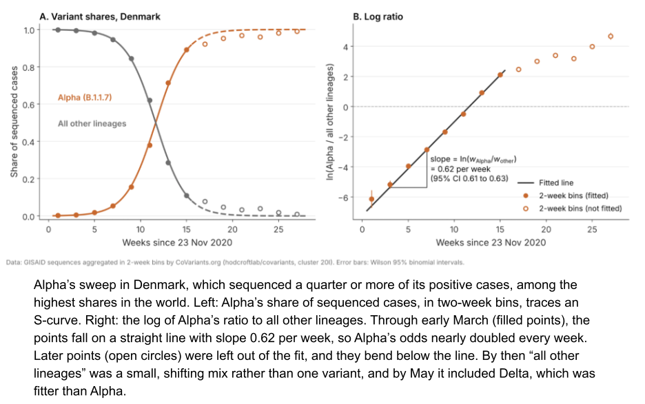
In January 2021, the Alpha variant of SARS-CoV-2 made up less than half a percent of US cases. The CDC projected that it would become the dominant variant by March (Galloway et al. 2021). By early April, it was the most common lineage in the US. The forecast didn’t need information about immune systems or social networks. It just modeled how much faster Alpha spread than other SARS-CoV-2 variants.

This suffices because variants are self-replicators. Advantages in exponential growth compound. The replicator equation is a simple way to model such processes.

Evolution is usually told as a story about DNA, but the replicator equation never mentions nucleic acid. The natural world is rife with many other replicators, and the replicator equation applies to all of them.

This post develops the replicator equation in its simplest form, and then relaxes its assumptions. We allow fitness to change, mutation to add new variants, and finally finite populations to introduce sampling. Each change can enrich the forecast.

Let’s dive in!

The Replicator Equation

A self-replicator makes more of itself, and each copy makes copies of its own. This entails positive feedback: the more copies exist, the faster new ones appear. When every copy replicates at a fixed pace, the population undergoes exponential growth, doubling at regular intervals. We define fitness w as the number of copies that each replicator leaves per generation.

Consider two strains of E. coli in a flask. Let’s suppose strain A has a doubling time of 30 minutes, and strain B has 20 minutes. All cells replicate at the rate prescribed by their strain identity. The strain of the parents is transmitted to their offspring. Each strain therefore breeds true.

A class of individuals that shares a fitness and breeds true is a variant. Not every class qualifies. “Large cells” does not breed true, because a large cell divides into two small ones. “All cells in the flask” breeds true, but its members do not share the same fitness. In sexually reproducing organisms, a genotype does not breed true, because sex reshuffles the genome.

Heritable state is whatever makes an offspring resemble their parent. In clonal bacteria, the heritable state is the genome. In sexual species, it is the allele. Heritable state can also be the composition of a chemical network, or a handwritten note.

Each variant i multiplies by its own fitness wᵢ every generation. Both strain populations grow. But strain B’s fraction of the flask grows toward 100%. More generally, the frequency $xᵢ = nᵢ/N$ obeys the replicator equation:

$x_i’ = x_i\frac{w_i}{\bar{w}}$

Here $w̄ = Σⱼxⱼwⱼ$ is the mean fitness and the factor $wᵢ/w̄$ is the relative fitness of the variant. A variant grows when it is fitter than average and shrinks when it is less fit.

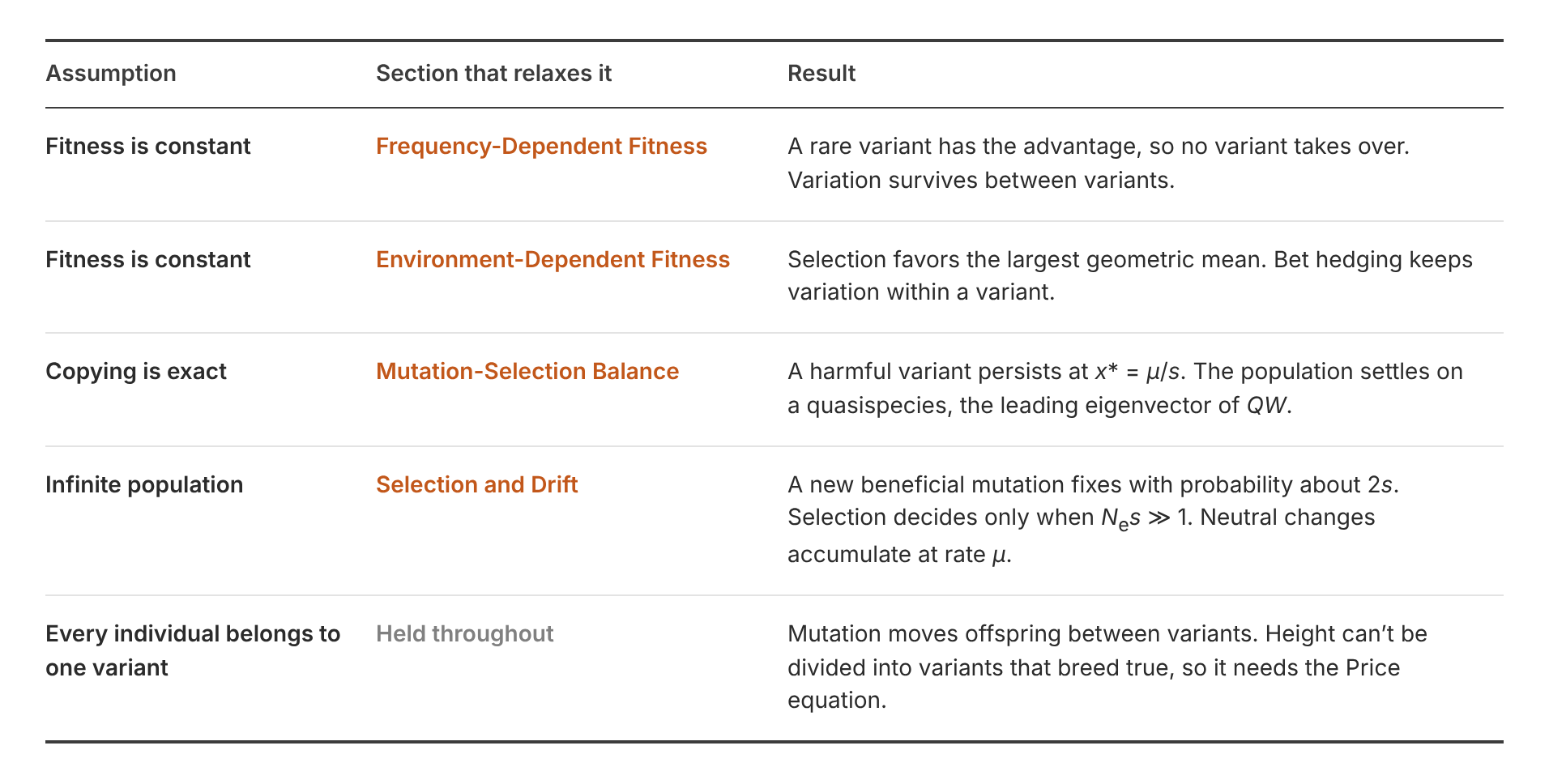
The replicator equation makes four assumptions:

1. Fitness is constant.
2. Copying is exact. Every offspring inherits the variant of its parent.
3. An infinite population. This entails no genetic drift.
4. Every individual belongs to exactly one variant.

The replicator equation describes real selective sweeps, with a fitter variant replacing its rivals. Each generation multiplies the odds of variant 1 against variant 2 by $w₁/w₂$:

$\ln\frac{x_1′}{x_2′} = \ln\frac{x_1}{x_2} + \ln\frac{w_1}{w_2}$

Mean fitness cancels, so only fitness ratios matter. On a plot of frequency, a variant with higher relative fitness traces an S-curve. On a plot of log ratio, it traces a straight line.

Under these assumptions, the fittest variant takes over: the variation disappears. Selection consumes the variation it runs on.

Frequency-Dependent Fitness

The replicator equation assumes that fitness is constant. When fitness changes, variation can survive.

The replicator equation assumes exponential growth, the case p = 1 in

$\frac{dn}{dt} = k n^p$

Szathmáry (1991) named the three cases.

• Parabolic growth (p < 1) gives survival of everybody. Fitness knᵖ⁻¹ falls as a variant becomes common, so rare variants outgrow common ones and none takes over. Growth at the edge of a colony is parabolic. So were the first synthetic template replicators, because each copy stays paired with its template and slows further copying (von Kiedrowski 1986).
• Exponential growth (p = 1) gives survival of the fittest. Fitness is constant, so the variant with the largest k takes over.
• Hyperbolic growth (p > 1) gives survival of the first. As a variant becomes common, its fitness rises. This allows an early variant to stay ahead, even against a more fit newcomer.

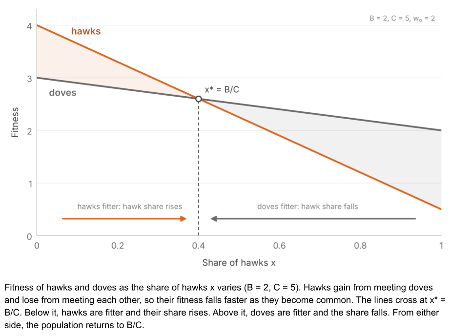
Fitness can also depend on the composition of the population. In the hawk–dove game (Maynard Smith & Price 1973; Maynard Smith 1982), two animals contest a prize worth B. Hawks fight, and the loser pays C. Doves share with doves and retreat from hawks. Each entry is the row player’s expected payoff against the column player:

$\begin{array}{c|cc} & \text{Hawk} & \text{Dove} \\ \hline \text{Hawk} & \frac{B-C}{2} & B \\ \text{Dove} & 0 & \frac{B}{2} \end{array}$

When a fight costs more than the prize ($C > B$), hawks do well among doves and badly among hawks. Let x be the share of hawks, and let each animal meet a random opponent. Each strategy’s fitness is a baseline w₀ plus its average payoff, so the hawks’ advantage

$w_H – w_D = x\frac{B-C}{2} + (1-x)\frac{B}{2} = \frac{B-xC}{2}$

This advantage is positive while hawks are rarer than $B/C$ and negative once they are more common. Each strategy does best when it is rare. The population settles where hawks make up $B/C$ of it. Evolutionary game theory develops such games in more detail.

Ecology has a well-known counterpart. Competitive exclusion (Gause 1934) states that two species limited by one resource cannot coexist. Species escape it when each limits its own growth more than it limits the other’s, so that each species has an advantage when rare (Chesson 2000).

The two models are one system in different coordinates. When fitness depends linearly on frequencies, the continuous-time replicator equation for n variants (Taylor & Jonker 1978) becomes the Lotka–Volterra equations for n − 1 species (Hofbauer 1981).

Environment-Dependent Fitness

Fitness can also depend on the environment, so that wᵢ is a function of time. Then the forecast must average over good years and bad ones, and the right average is not the obvious one.

Consider a desert annual plant. Rain falls in 75% of years ($π = 0.75$). In a rainy year, a plant makes two seeds ($w_{rain} = 2$). In a dry year, the plant leaves 0.1 seeds on average ($w_{dry} = 0.1)$. Let’s assume that the climate is unpredictable. Let one year be one generation.

Let each member of variant i leave $wᵢ(t)$ offspring in year t. After T years, its lineage has grown by the product of these fitnesses. The geometric mean fitness Gᵢ is the constant yearly fitness that produces the same growth:

$G_i = \left(\prod_{t=1}^{T} w_i(t)\right)^{1/T}$

So each lineage grows by $Gᵢᵀ$, and the variant with the largest G takes over.

Taking the log turns the product into an average, the same form as the arithmetic mean fitness Aᵢ:

$A_i = \frac{1}{T}\sum_{t=1}^{T} w_i(t) \to E[w_i]$

$\ln G_i = \frac{1}{T}\sum_{t=1}^{T} \ln w_i(t) \to E[\ln w_i]$

As T grows, both averages approach these limits when each year’s environment is drawn independently from a fixed distribution. Because ln G approaches $E[ln(w)]$, selection favors the variant with the largest expected log fitness.

For the desert annual that germinates every seed:

$A = \pi w_{\text{rain}} + (1-\pi) w_{\text{dry}} = 0.75 \times 2 + 0.25 \times 0.1 \approx 1.53$

$G = w_{\text{rain}}^{\pi} \times w_{\text{dry}}^{1-\pi} = 2^{0.75} \times 0.1^{0.25} \approx 0.95$

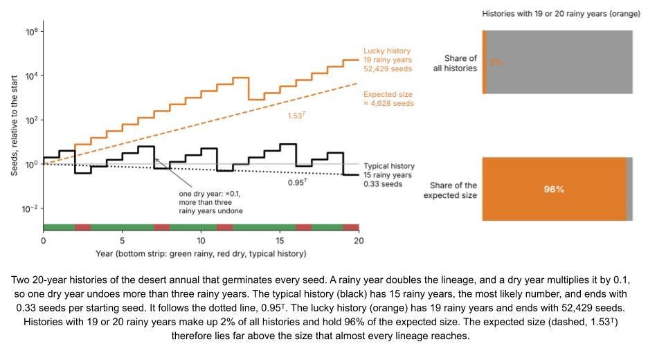
Recall that a plant leaves 2.0 or 0.1 seeds depending on the rain. Scaling by the natural log, a rainy year adds 0.69 and a dry year subtracts 2.30 fitness. A dry year cancels the effect of more than three rainy years! This result derives from Jensen’s inequality where, for any concave function f,

$E[f(x)] \le f(E[x])$

Since logarithms are concave:

$\underbrace{E[\ln w]}_{\ln G} \le \underbrace{\ln E[w]}_{\ln A}$

So G < A whenever fitness varies.

The means answer different questions. The arithmetic mean is an ensemble average: lineage size across every possible sequence. The geometric mean is a time average, lineage size across very long experiences of a single variant. Ergodicity holds when ensemble and time averages agree (Peters & Gell-Mann 2016).

Compounding growth lacks ergodicity, so the arithmetic mean misleads. Lewontin & Cohen (1969) showed that a population like our desert annual can grow in expected size, while its extinction is almost certain.

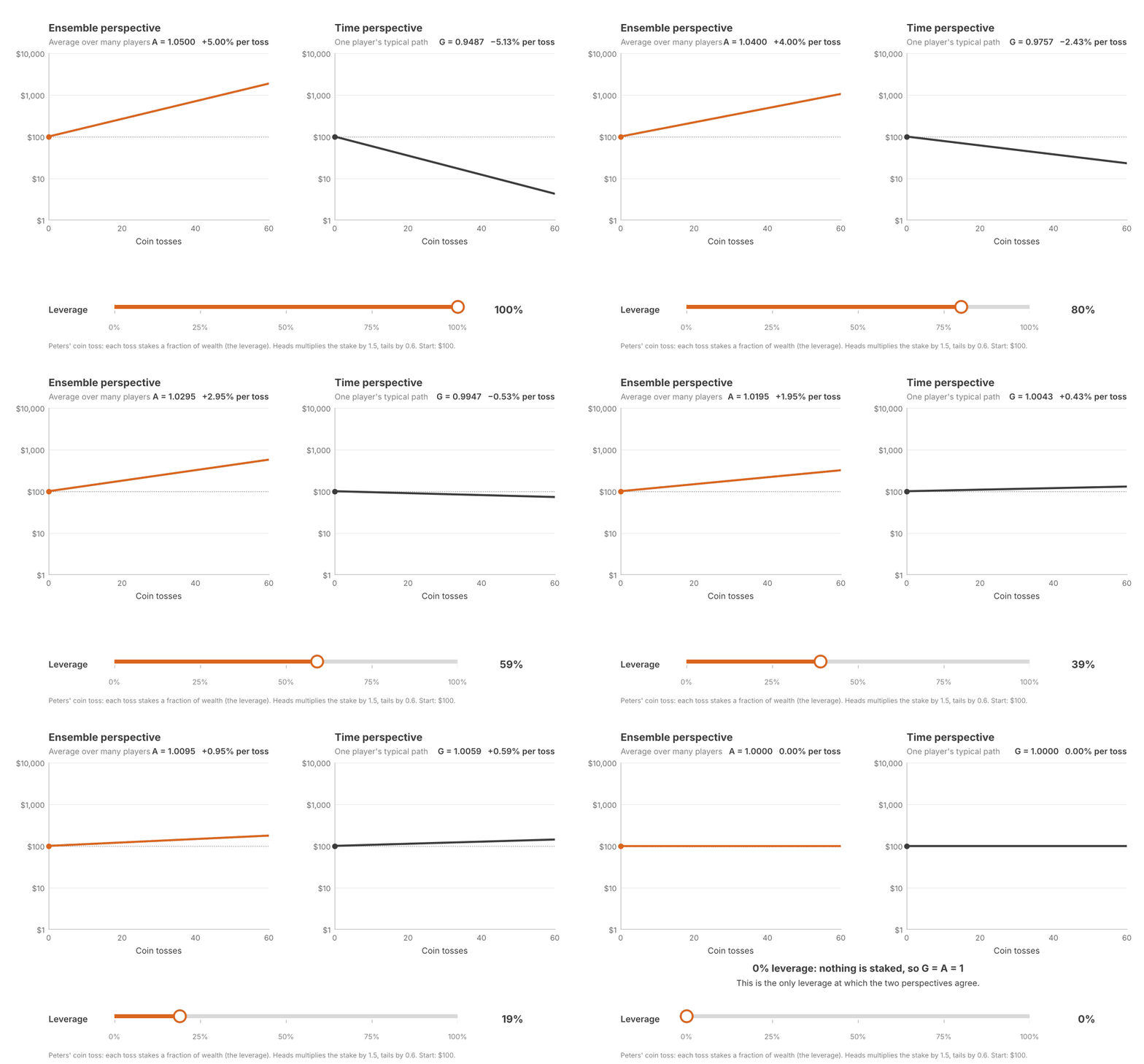
Finance also features exponential growth. In that field, this phenomenon is called volatility drag: an investment with a positive average return can lose money in almost every history. Peters & Gell-Mann (2016) use a coin toss. Each toss stakes a fraction of wealth, the leverage; heads multiplies the stake by 1.5 and tails by 0.6. More leverage always raises A. G rises only until 25% leverage, then falls, and drops below 1 past 50%. The Kelly criterion (Kelly 1956) chooses the leverage that maximizes G, here 25%. Selection, like the Kelly bettor, maximizes G.

Hedging, Plasticity, and Tracking

An organism can respond to a fluctuating environment in three ways (Botero et al. 2015).

1. Fast change with no reliable cue favors bet hedging.
2. Fast change with a reliable cue favors plasticity.
3. Slow change favors tracking by selection.

Bet hedging gives up some success in good years to reduce losses in bad years (Seger & Brockmann 1987). It takes two forms. In conservative bet hedging, everyone adopts a safe phenotype that consistently does moderately well. Gorillas prefer fruit, but fall back on vegetation when it is scarce (Marshall & Wrangham 2007). Every gorilla maintains a gut capable of processing those fallback foods. This tissue demands continual maintenance, but pays off in years when fruit fails.

A desert annual could hedge the same way. Imagine a hardy plant leaving 1.4 seeds in a rainy year and 0.5 in a dry year. Its lineage grows:

$A = 0.75 \times 1.4 + 0.25 \times 0.5 \approx 1.18$

$G = 1.4^{0.75} \times 0.5^{0.25} \approx 1.08$

In diversified bet hedging, one genotype produces offspring of several phenotypes. Desert annuals are a classic case. Each year some of their seeds germinate and the rest stay dormant in the soil (Cohen 1966). A dormant seed survives the year and leaves itself, so it scores 1 in every year. Neither phenotype does well alone. A lineage that always germinates shrinks, and a lineage that always stays dormant never grows. A lineage that germinates 60% of its seeds leaves 1.60 seeds in a rainy year and 0.46 in a dry year. This diversified approach outperforms our hypothetical conservative hedge:

$A = 0.75 \times 1.60 + 0.25 \times 0.46 \approx 1.32$

$G = 1.60^{0.75} \times 0.46^{0.25} \approx 1.17$

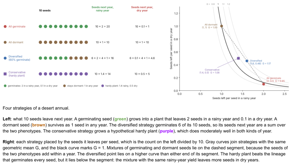
Diversified hedging can look like the hawk–dove mix, which a population can reach in two ways: every animal plays hawk with probability B/C (a mixed strategy), or a fraction B/C always plays hawk (a polymorphism). Against the weather, only the mixed strategy works. In a polymorphism, the always-germinating and never-germinating seeds form separate lineages, and the dormant one takes over.

Suppose a seed could tell in advance whether a year will be rainy. It could outperform even the best hedging strategy. When a cue such as soil moisture or temperature reliably forecasts environmental conditions, an organism can develop the phenotype that matches the coming conditions. Biologists call this adaptive phenotypic plasticity. With a partly reliable cue, the best strategy combines plasticity and hedging (Cohen 1967).

When the environment changes slowly, over many generations, selection itself can follow it. A run of wet years favors one variant, and a later run of dry years favors another. Biologists call this adaptive tracking.

Mutation–Selection Balance

The replicator equation also assumes that copying is exact. But physical replication makes mistakes, and each error can create a new variant. This noise resupplies the variation that selection consumes. Mutation–selection balance denotes their equilibrium state.

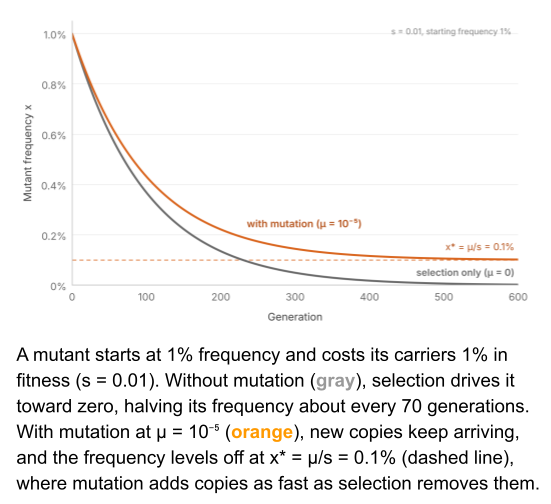
Consider a harmful variant in a haploid population. Let μ denote the mutation rate, and let’s ignore mutations back to the original for now. Let s denote the mutant’s fitness cost. In each generation, mutation adds about μ to the frequency x of the mutant, and selection removes about sx:

$\Delta x = \text{inflow} – \text{outflow} \approx \mu – s x$

The frequency stops changing when the two terms cancel:

$x^* \approx \frac{\mu}{s}$

Imagine a mutation rate of $μ = 10⁻⁵$. Mildly harmful variants of $s=0.01$ persist at ten times the frequency of more serious mutations of $s=0.1$. Weaker selection leaves a harmful variant more common. Imperfect copying entails a reservoir of harmful variants. But it also supplies the rare beneficial mutations that selection can spread.

Let’s generalize this to a vector of variant counts n. Selection multiplies each count by its fitness, through a diagonal matrix W. Copying moves offspring between variants, through a matrix Q whose entries $Qij$ give the probability that parent j will leave an offspring of variant i. One generation is

$n’ = QWn$

This is the replicator–mutator equation (Eigen 1971). Without mutation, Q is the identity matrix and the variant with the largest fitness takes over. With mutation, variants move towards an equilibrium mixture known as a quasispecies (Eigen & Schuster 1979).

Drift

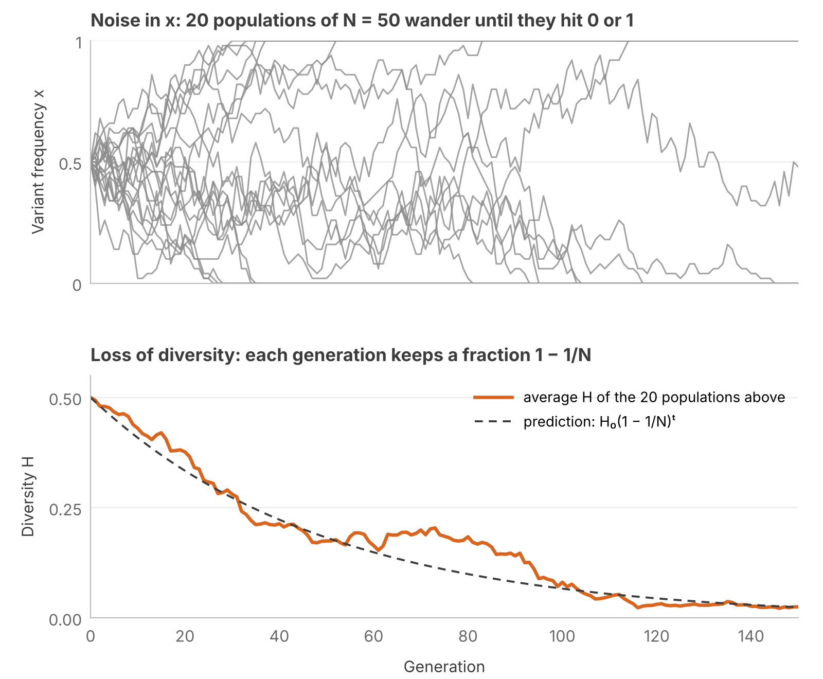
The replicator equation assumes an infinite population. But real populations are finite. Each generation is a sample of the last: offspring are drawn from the parents in proportion to their fitness. Sampling adds noise called drift, which shrinks as N grows. For a variant at frequency x in a population of N haploid individuals, the variance of the change in one generation is

$\operatorname{Var}(\Delta x) = \frac{x(1-x)}{N}$

Drift adds noise to frequencies. Ironically, this erodes variation within a population. Let H be the chance that two randomly drawn copies differ:

$H = 1 – \sum_i x_i^2$

Two copies are both variant i with probability $xᵢ²$, so the sum is the chance they match. In the left image below, H is the area of mismatches off the diagonal.

As a diversity metric, H is known as expected heterozygosity. It is a member of the entropy family, closely related to Shannon entropy.

Assume all fitness differences are insignificant. Drift removes diversity in three steps:

1. x wanders like a fair random walk: its expected step is zero, $E[Δx] = 0$, and its next step depends only on where it is now. Such a walk is called a martingale.
2. 0 and 1 are absorbing walls: once a variant is gone, only mutation can bring it back. So every population eventually hits a wall, and none ever leaves one.
3. Even before any wall is hit, fair steps lower H on average, because H is concave in x: the arch bends downward, so a step down its slope loses more H than an equal step up gains. This is the Jensen gap again, the one that pulls G below A.

With two variants, $H = 2x(1 − x)$ is a parabola, so its Taylor expansion stops at the $Δx²$ term:

$H(x + \Delta x) = H(x) + 2(1 – 2x)\,\Delta x – 2\,\Delta x^2$

Let $H′ = H(x + Δx)$denote the diversity of the next generation. We would like to know its expectation $E[H′]$: the expected outcome of drift over time.

$E[H’] = H + 2(1-2x)\,\underbrace{E[\Delta x]}_{0} – 2\,\underbrace{E[\Delta x^2]}_{\mathrm{Var}(\Delta x)} = H – 2\,\mathrm{Var}(\Delta x)$

Drift’s step variance then simplifies to:

$\mathrm{Var}(\Delta x) = \frac{x(1-x)}{N} = \frac{H}{2N}$

Putting the pieces together:

$E[H’] = H – \frac{H}{N} = H\left(1 – \frac{1}{N}\right)$

Without a source of new variants, drift pushes finite populations towards uniformity.

In these formulae, we’ve used N as population size. But drift doesn’t care about individuals who don’t reproduce. We require a notion of effective population size Nₑ. How to operationalize it?

Imagine tracing two gene copies back in time. This backward-facing perspective is called the coalescent (Kingman 1982). In a population of N haploid individuals, two copies share a parent with probability 1/N each generation, so on average they meet in a common ancestor N generations back. Small populations produce shallow family trees.

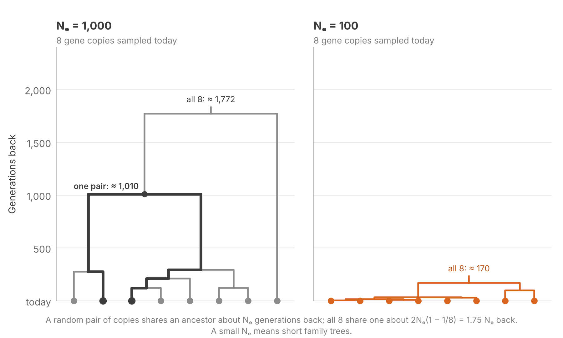
Let’s start by defining Nₑ as the size of an ideal population with the following property:

$P(\text{two copies share a parent}) = \frac{1}{N_e}$

We can upgrade this abstraction in two ways. First, let $σ²$ be the variance in offspring. In the ideal population, offspring numbers have $σ² = 1$. But reproductively unequal species can have very large $σ²$. This increases the probability that two copies trace back to the same parent.

$P(\text{two copies share a parent}) \approx \frac{\sigma^2}{N}$

Some marine species with sweepstakes reproduction have Nₑ thousands of times smaller than their census size (Hedgecock & Pudovkin 2011).

Second, let us countenance changes in population size. Define Nₜ as the census size of parents in generation t, and σₜ² as offspring variance. Two copies share a parent with probability $pₜ = σₜ²/Nₜ$, and miss with probability $1 − pₜ$. For two copies to not share a parent, they must miss each generation. Nₑ is the constant effective size that gives the same probability:

$\left(1 – \frac{1}{N_e}\right)^{T} = \prod_{t=1}^{T} \left(1 – p_t\right)$

$T \ln\left(1 – \frac{1}{N_e}\right) = \sum_{t=1}^{T} \ln\left(1 – p_t\right)$

For a small chance p, $ln(1 − p) ≈ −p$, so

$\frac{1}{N_e} \approx \frac{1}{T}\sum_{t=1}^{T} p_t = \frac{1}{T}\sum_{t=1}^{T} \frac{\sigma_t^2}{N_t}$

Nₑ is therefore the harmonic mean of each generation’s Nₜ/σₜ². Population bottlenecks can dominate the harmonic mean. Three generations of 1,000, 1,000 and 10 breeders with σ² = 1 give Nₑ ≈ 29: one crash outweighs many generations of plenty. Humans number in the billions, but our Nₑ is about 10,000 to 20,000 individuals, because for most of our history we were few.

Selection, Drift and Mutation

With our new understanding of drift, let’s reintroduce mutations and selection.

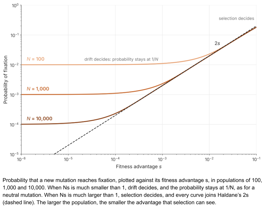
Drift is hardest on new mutations. A single new mutation with fitness advantage s is easy to lose. Haldane (1927) showed that it only reaches fixation with probability about 2s. A mutation that raises fitness by 1% is lost 98% of the time.

Kimura (1962) showed that drift and selection operate at different timescales. Selective sweeps take effect over about 1/s generations. Drift needs about Nₑ generations to bring a variant to an absorbing wall. Putting these together:

$\frac{\text{drift time}}{\text{selection time}} \approx \frac{N_e}{1/s} = N_e s$

When $Nₑs$ is much smaller than 1, drift moves the variant before selection can. When it is much larger than 1, selection wins. Kimura’s formula joins the two regimes to capture the probability of fixation:

$P_{\text{fix}} \approx \frac{1 – e^{-2s}}{1 – e^{-2N_e s}}$

Consider two copies.

• Mutation refills diversity at a rate of 2μ.
• Selection drains diversity at a rate of s.
• Drift drains diversity at a rate of 1/Nₑ.

Diversity H settles where inflow equals outflow:

$H^* \approx \frac{2\mu}{s + 1/N_e}$

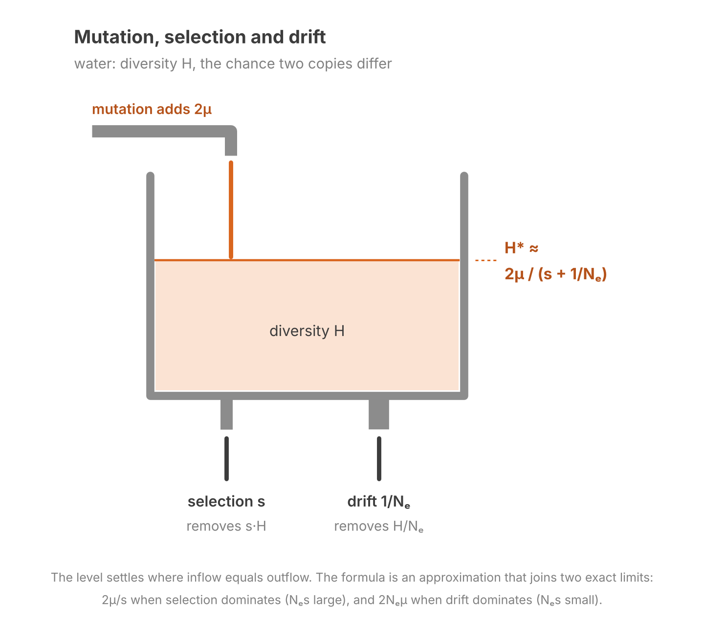
When $Nₑs ≫ 1$, drift is irrelevant and the mutation–selection balance operates. When $Nₑs ≪ 1$, selection is irrelevant and the mutation–drift balance operates.

Drift also keeps time. A population of N haploid individuals gains about $Nμ$ new neutral mutations each generation, and each one reaches fixation with a probability equal to its starting frequency, 1/N. The population size cancels:

$k = N\mu \times \frac{1}{N} = \mu$

Neutral substitutions therefore accumulate at the mutation rate, whatever the size of the population (Kimura 1968), and biologists use this molecular clock (Zuckerkandl & Pauling 1965) to date the divergence of lineages from the differences between their sequences.

When beneficial mutations are rare, a population adapts one selective sweep at a time. Each new mutation survives drift with probability about 2s, then spreads along the S-curve of the replicator equation (Gillespie 1984).

Applications

Faced with a new replicator, people first ask its doubling time. But two other questions pertain. Does its fitness fall once it is common, and does it carry a heritable state that can change? Let’s apply these questions to three examples.

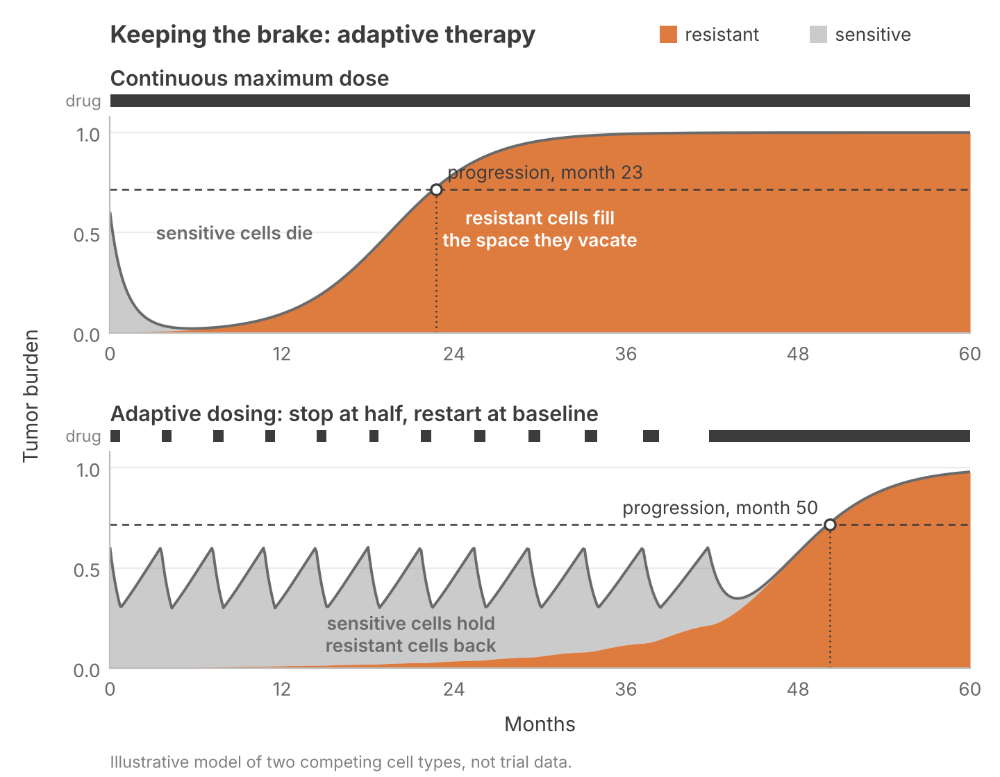
First, drug-sensitive and drug-resistant tumor cells compete for the same nutrients. Treatment at the maximum dose kills the sensitive cells. But this produces a competitive release: it hands the tumor to the resistant cells. Adaptive therapy pauses the drug before the sensitive cells are gone, so they continue to suppress their rivals (Zhang et al. 2017). In a pilot trial of 11 men with metastatic prostate cancer, median time to progression was at least 27 months, against 16.5 months on standard dosing.

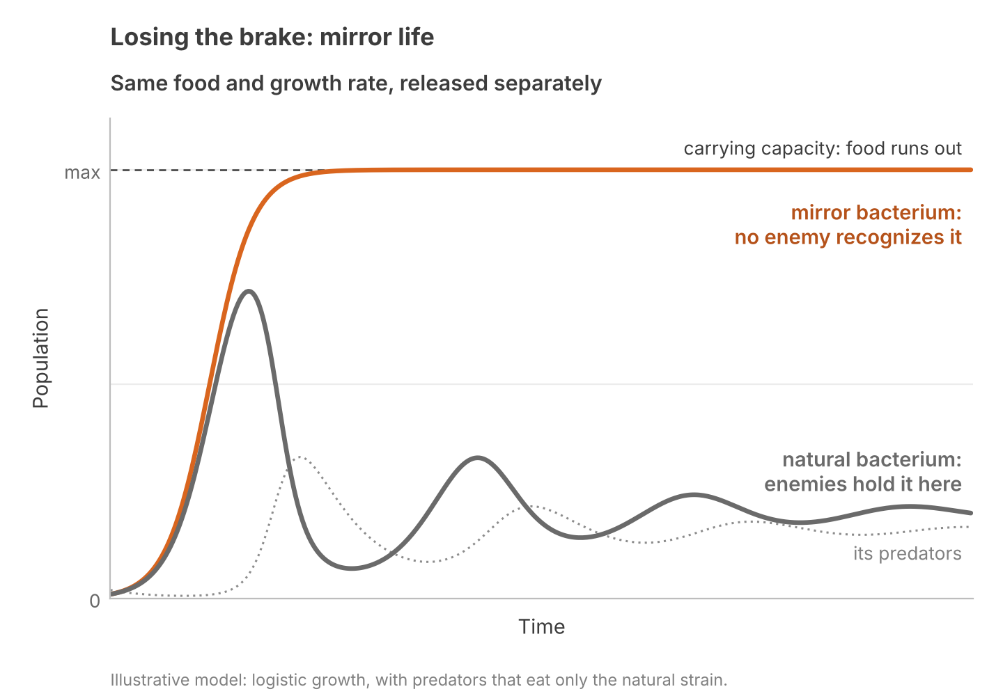
Second, let’s consider mirror life. During abiogenesis and for mysterious reasons, life on Earth became homochiral. Geochemistry produces racemic molecules, with equal proportions of right and left-handed configurations. But proteins use only left-handed amino acids and DNA only right-handed sugars. A mirror bacterium could be built with proteins and nucleic acids of the opposite handedness, and it would likely replicate at similar rates.

Mirror life is dangerous for other reasons. In conventional life, predators hold populations far below the carrying capacity of the environment. But predators recognize their prey by molecular shape, so a mirror bacterium could grow without these constraints (Adamala et al. 2024). Ecologists call this enemy release.

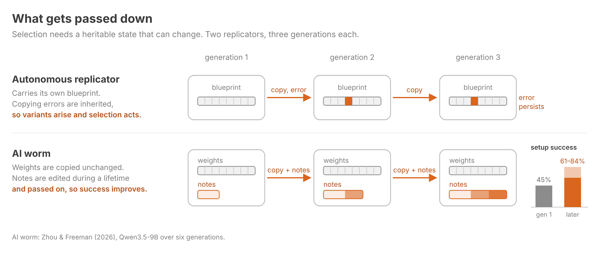
Finally, consider replicating software. Many botnets are spread from a central server, which nanotechnologists call a broadcast architecture (Phoenix & Drexler 2004). For example, Mirai doubled in size every 76 minutes (Antonakakis et al. 2017). But these bots are duplicated exactly, so selection has nothing to act on.

Zhou & Freeman (2026) asked whether open-weight LLMs could spread across consumer devices such as TV boxes and phones. As of October 2026, no such worm exists. In their sandbox, each LLM took 1–2 days to replicate. But despite having identical weights, this AI botnet was able to improve across generations. With each instance leaving notes for its successor, setup success rose from 45% to 61–84% in later generations. These notes constitute a heritable state.

Doubling time constrains how a replicator starts. Our other questions reveal where it ends.

Relation to Prior Work

In 2015, I wrote three posts which build intuitions on the same material.

Intro to Population Genetics described evolution with spatial metaphors. A genotype is a location in gene space, an organism is a point, and a species is a cluster of points. The replicator equation quantifies movement in this space. The frequency xᵢ is the fraction of the cluster’s points at location i. Mutation places a child one step from its parent. Genetic drift is the random travel of the whole cluster. A population that passes through a bottleneck takes large steps. The 2015 post also asked the reader to treat the population, and not the individual, as the actor. The replicator equation mathematically formalizes that view.

Intro to Natural Selection added height to this space: fitness. Here we pictured selection as uphill locomotion on a fitness landscape. When fitness is constant, the replicator equation climbs a related landscape, whose points are populations and whose height is mean fitness. The sections of this post explain the features of the 2015 picture. Selection only reweights points that already exist, so a population reaches new genotypes by mutation. When mutations are rare, it climbs one sweep at a time. Mutation–selection balance sets how widely the population spreads around a peak. A slope gentler than about 1/Nₑ is flat in practice.

Fitness Seascapes grounded fitness in energy. An environment can support only a finite population, its carrying capacity, and a population at carrying capacity has mean fitness 1. The replicator equation is consistent with this. Relative fitness drives change, so the competition is zero-sum. One variant’s gain is another’s loss. This is the basis for my 2015 description of fitness as a finite resource. I also noted that the landscape differs from one habitat to the next and called it a seascape. Environment-dependent fitness is that seascape changing in time, and bet hedging and adaptive tracking are two ways to live on it.

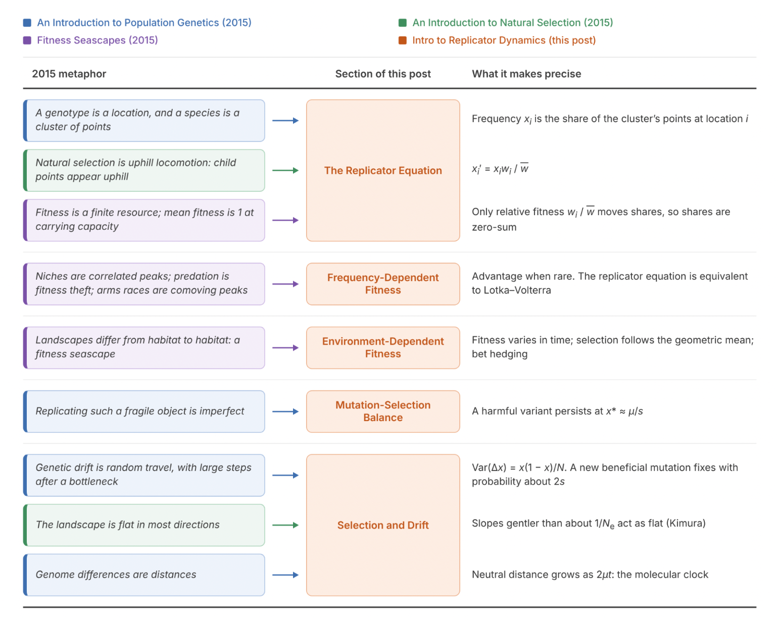
The previous posts described gene space, the space of DNA sequences. Today’s post generalizes it to a space of heritable states, which matters most for the origin of life. Its theories propose replicators of many kinds, from autocatalytic sets of small molecules to self-copying RNA.

Wrapping Up

This post relaxed three of the replicator equation’s four assumptions.

Each assumption we relaxed had consequences.

1. Fitness can change in two ways. Frequency dependence keeps rivals alive. A fluctuating environment can favor variety among one parent’s offspring.
2. Finite populations entail drift. Like selection, drift erodes variation. In small populations, drift can overwhelm selection that would win in a larger population.
3. Imperfect copying entails mutation. Mutation is the source of variation needed to keep the engines of selections and drift running.

One assumption held throughout this post: that every individual belongs to exactly one variant. Variant partitions require access to heritable state. But we can measure a giraffe’s neck without knowing which of thousands of alleles shaped it. It would be nice to reason directly about the fitness of phenotypes.

Next time, we will relax this assumption and work with measurements directly. See you then!

References

1. Adamala et al. (2024). Confronting risks of mirror life.
2. Antonakakis et al. (2017). Understanding the Mirai botnet.
3. Botero et al. (2015). Evolutionary tipping points in the capacity to adapt to environmental change.
4. Chesson (2000). Mechanisms of maintenance of species diversity.
5. Cohen (1966). Optimizing reproduction in a randomly varying environment.
6. Cohen (1967). Optimizing reproduction in a randomly varying environment when a correlation may exist between the conditions at the time a choice has to be made and the subsequent outcome.
7. Eigen (1971). Selforganization of matter and the evolution of biological macromolecules.
8. Eigen & Schuster (1979). The Hypercycle: A Principle of Natural Self-Organization.
9. Galloway et al. (2021). Emergence of SARS-CoV-2 B.1.1.7 lineage — United States, December 29, 2020–January 12, 2021.
10. Gause (1934). The Struggle for Existence.
11. Gillespie (1984). Molecular evolution over the mutational landscape.
12. Haldane (1927). A mathematical theory of natural and artificial selection, Part V: Selection and mutation.
13. Hedgecock & Pudovkin (2011). Sweepstakes reproductive success in highly fecund marine fish and shellfish: a review and commentary.
14. Hofbauer (1981). On the occurrence of limit cycles in the Volterra–Lotka equation.
15. Kelly (1956). A new interpretation of information rate.
16. Kimura (1962). On the probability of fixation of mutant genes in a population.
17. Kimura (1968). Evolutionary rate at the molecular level.
18. Kingman (1982). The coalescent.
19. Lewontin & Cohen (1969). On population growth in a randomly varying environment.
20. Marshall & Wrangham (2007). Evolutionary consequences of fallback foods.
21. Maynard Smith (1982). Evolution and the Theory of Games.
22. Maynard Smith & Price (1973). The logic of animal conflict.
23. Peters & Gell-Mann (2016). Evaluating gambles using dynamics.
24. Phoenix & Drexler (2004). Safe exponential manufacturing.
25. Seger & Brockmann (1987). What is bet-hedging?
26. Szathmáry (1991). Simple growth laws and selection consequences.
27. Taylor & Jonker (1978). Evolutionarily stable strategies and game dynamics.
28. von Kiedrowski (1986). A self-replicating hexadeoxynucleotide.
29. Zhang et al. (2017). Integrating evolutionary dynamics into treatment of metastatic castrate-resistant prostate cancer.
30. Zhou & Freeman (2026). AI models may be capable of self-replicating without access to a datacenter.
31. Zuckerkandl & Pauling (1965). Evolutionary divergence and convergence in proteins.