Part Of: Probability Theory sequence
Content Summary: 1000 words, 10 min read

Describing Depression

In An Introduction To Bayesian Inference, you were introduced to the discrete random variable:

You remember algebra, and how annoying it was to use symbols that merely represented numbers? Statisticians get their jollies by terrorizing people with a similar toy, the random variable. The set of all possible values for a given variable is known as its domain.

Let’s define a discrete random variable called Happy. We are now in a position to evaluate expressions like Probability(Happy=true)

The domain of Happy is of size two (it can resolve to either true, or false). Since domain size is pivotal in this post, we will abbreviate it. Let an Variable_N be a discrete random variable whose domain is size N (in the literature, the probability distribution for Variable_N is known as the categorical distribution).

Consider a new variable, Emotion₂ = { happy, sad }. Suppose we use this variable to describe a person undergoing a major depression. At any one time, such a person may have a 25% chance of being happy, and a 75% chance of being sad. This state of affairs can be described in two ways:

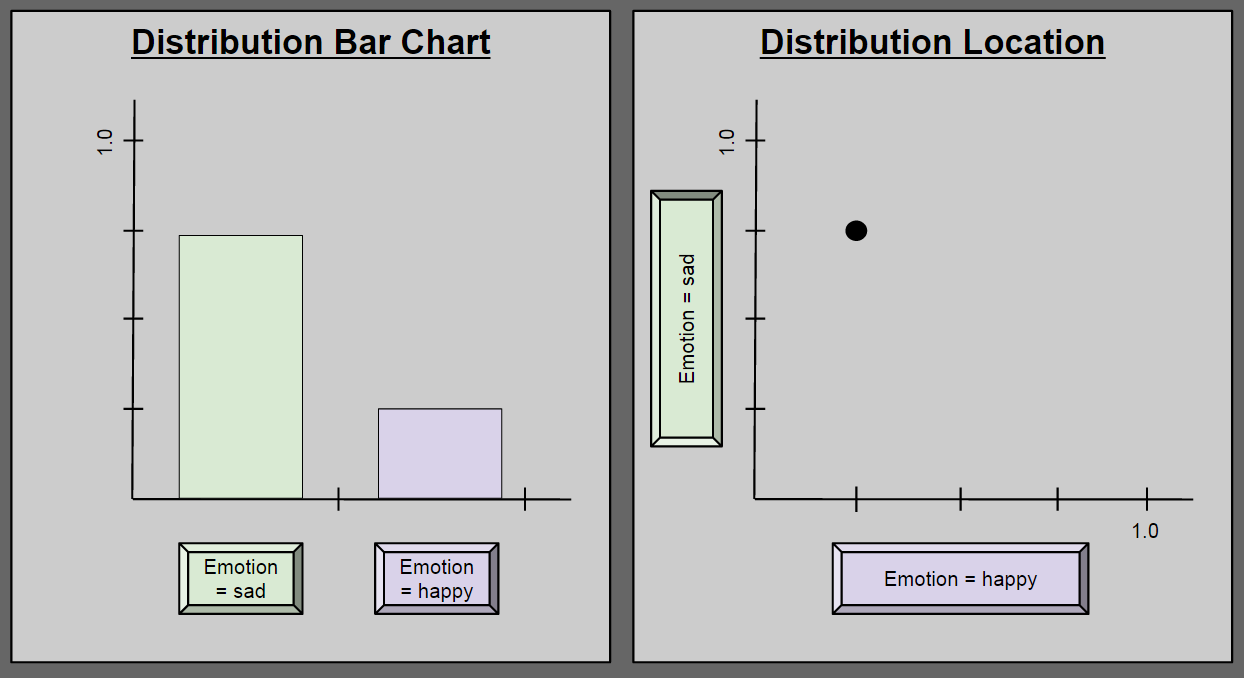
Pause here until you can explain to yourself why these diagrams are equivalent.

A Modest Explanation Of All Emotion

We have seen how a particular configuration of Emotion₂ can accurately characterize a depressed person. But Emotion₂ is intended to describe all possible human emotion. Can it take on any value in this two-dimensional space? No: to describe a human being as P(happy) = 1.5; P(sad) = -0.1 is nonsensical. So what values besides (0.25, 0.75) are possible for Emotion₂?

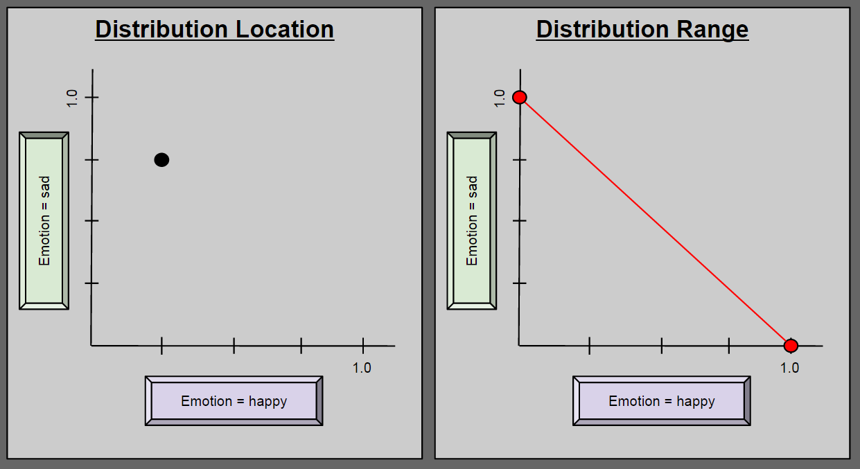
The above range diagram (right side) answers our question: any instance of Emotion₂ must reside along the red line. Take a second to convince yourself of this. It sometimes helps to think about the endpoints (0.0, 1.0) and (1.0, 0.0).

Bar Charts Are Hyperlocations

Perhaps you are not enthralled with the descriptive power of Emotion₂. Perhaps you subscribe to the heresy that certain human experiences cannot be usefully described as either happy or sad. Let us expand our model to catch these “corner cases”, and define Emotion₃ = { happy, sad, other }.

Can we identify a distribution range of this new variable? Of course!

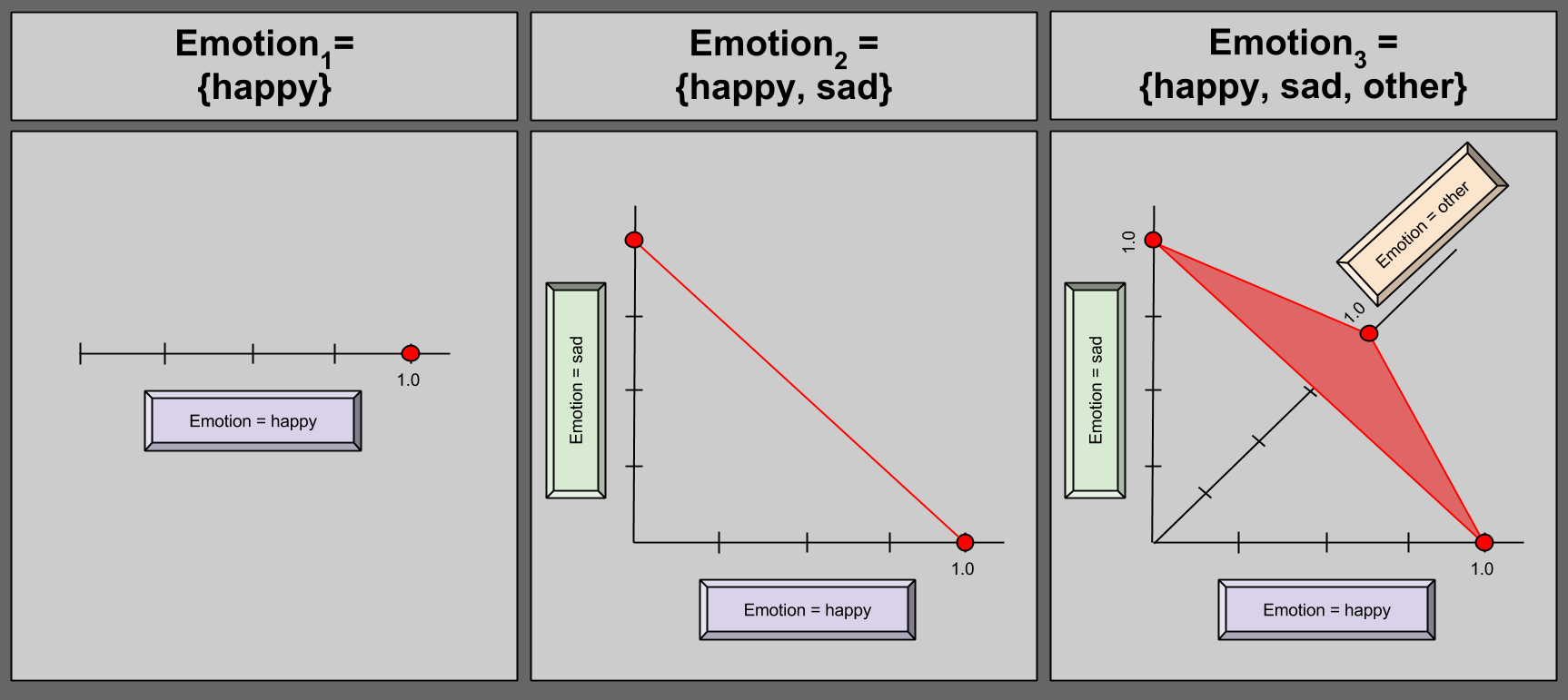
Take a moment to convince yourself that Emotion₃ may never contain any point outside the shaded red area.

Alright, so we have a fairly pleasing geometric picture of a discrete random variables with domains up to size 3. But what happens when we mature our model again? Imagine expanding our random variable to encapsulate the six universal emotions.

Could you draw a bar chart for an arbitrary Emotion₆?

Of course you could; you’d simply need to add four more bars to the first diagram of this post.

Now, what about location in space?

Drawing in 6-D is hard. 🙂

Here is the paradox: a simple bar chart corresponds with a cognitively intractable point in 6-dimensional space. I hope you never look at bar charts the same way!

An aside that, despite the constant three being sloppily hardcoded into our mental software, it turns out that reasoning about hyperlocations – points in N-dimensional space – is an important conceptual tool. If I ever get around to summarizing Drescher’s Good and Real, you’ll see hyperlocations used to establish an intuitive guide to quantum mechanics!

Miserly Description

But do we really need 6-dimensional space to describe a domain of size 6? Perhaps surprisingly, we do not. Consider the case of Emotion₃ = {happy, sad, other} again. Suppose I give you P(happy) = 0.5; P(sad) = 0.2. Do you really need me to tell you the P(other) = 0.3?

You could figure this out on your own, because the remaining 30% has to come from somewhere (0.3 = 1.0 – 0.5 – 0.2).

Given this fact that a variable has a 100% chance of being something (aka unitarity), we can describe a 4-variable in 3 dimensions:

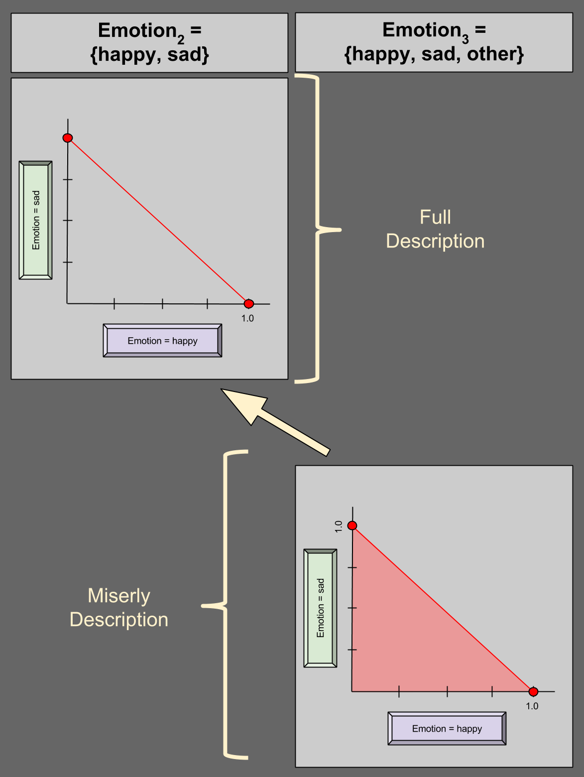
In the bottom-right of the diagram, we see an illustration of miserly description. Suppose we are given (0.25, 0.25) for happy and sad, respectively. P(other) must then be valued at 0.5, and (0.25, 0.25) is thus a valid distribution – this is confirmed by its residence in the shaded region above. Suppose I give you any point on the dark red edge of the region (e.g., (1.0, 0.0)); what value for P(other) must you expect? Zero.

This generalizes: unitarity allows us to describe an N-variable in N-1 dimensions. Here are two more examples:

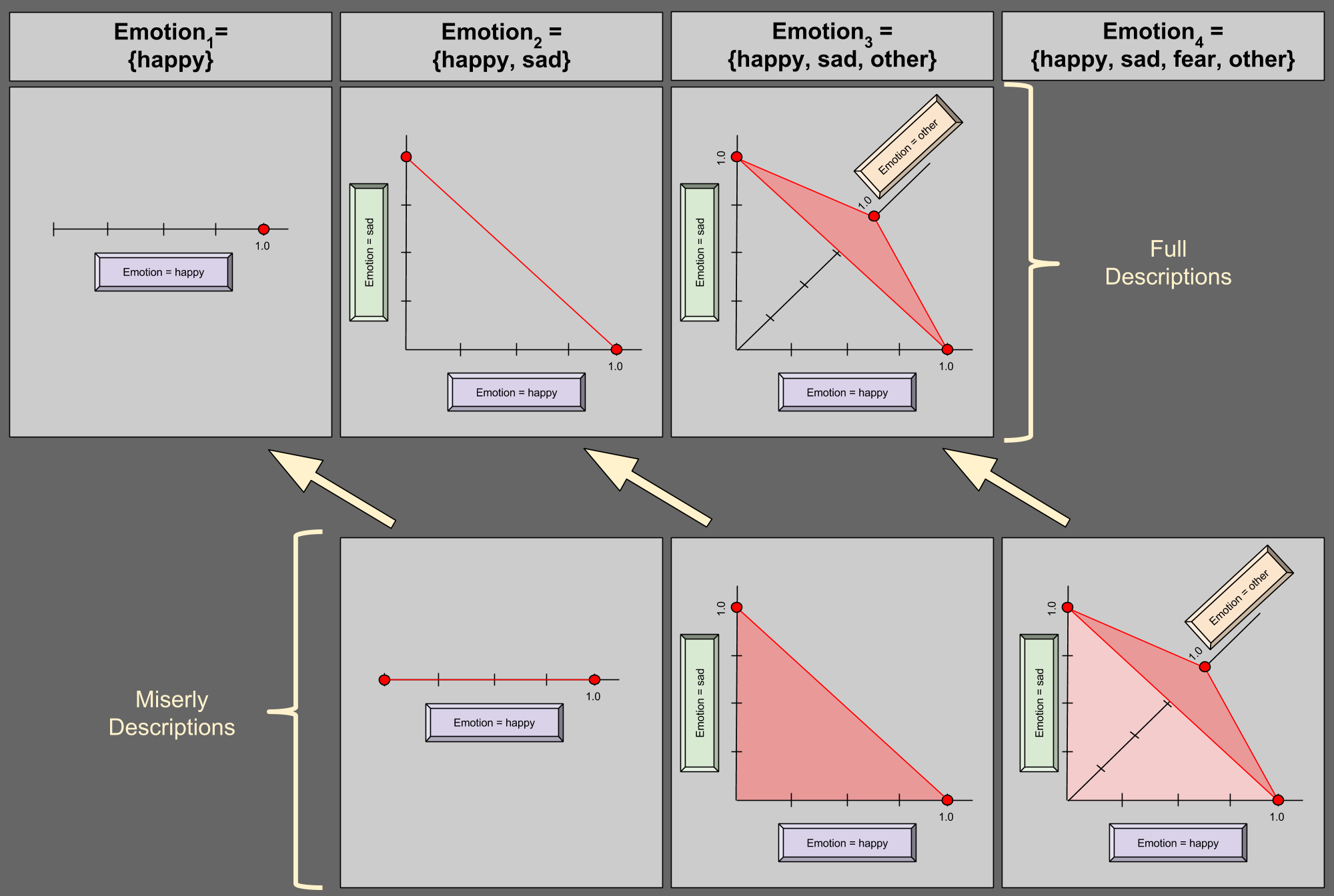
Notice the geometric similarities between the two descriptive styles, denoted by the yellow arrows.

The Hypervolume Of Probability

Consider the bottom row of our last figure (miserly descriptions). These geometric objects look similar: a triangle is not very different from a tetrahedron. What happens when we again move into a higher-dimensional space? Well, it turns out that there’s a name for this shape: a simplex is a generalization of a triangle into arbitrary dimensions. Personally, I would have preferred the term “hyperpyramid”, but I suppose the book of history is shut on this topic. 😛

We have thus arrived at an important result. The probability distribution associated with a discrete random variable can be represented as a simplex.

A Link To Convexity

I want you to recall my discussion on convex combinations.

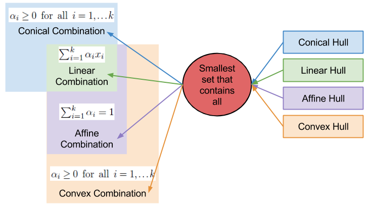
A convex combination should smell a lot like a probability distribution. Consider the axioms of Kolmogorov’s probability theory:

1. The probability of an event is a non-negative real number.
2. The probability that some event in the entire sample space will occur is 1.0
3. The probability of the intersection of several events is equal to the sum of their individual probabilities.

If you compare these axioms to the maths of the above combinations, and squint a little, you’ll begin to hypothesize similarities. 🙂

It turns out simplices form a bridge between convex hulls and probability distributions, because a simplex simply is a convex hull.

Takeaways

• Discrete random variables can refer to domains with more than two events.
• As a description, a bar chart is interchangeable with a hyperlocation.
• The range of possible probability distributions is relatively easy to characterize
• We can describe one fewer dimension of a distribution by leveraging the fact of unitarity.
• Such “miserly descriptions” reveal that all possible probability distributions of a categorical random variable is a generalized triangle (a simplex).
• This geometric result reveals a deep connection between the foundations of probability theory and convex analysis.