golden ratio | Fewer Lacunae

Part Of: Algebra sequence
Followup To: An Introduction to Linear Algebra
Next Up: Singular Value Decomposition
Content Summary: 1300 words, 13 min read

Geometries of Eigenvectors

Matrices are functions that act on vectors, by mapping from row-vectors to column-vectors. Consider two examples:

Reflection matrices, which reflect vectors across some basis.
Rotation matrices, which rotate vectors clockwise by $\theta$ degrees.

eigenvectors-transformation-geometries-1

The set of eigenvectors of a matrix $A$ is a special set of input vectors for which the matrix behaves as a scaling transformation. In other words, we desire the set of vectors $\vec{x}$ whose output vectors $A\vec{x}$ differ by a scaling factor.

Eigenvectors have a straightforward geometric interpretation:

Reflection eigenvectors are orthogonal or parallel to the reflecting surface. In the left image above, that is the top two pairs of vectors.
Rotation eigenvectors do not exist (more formally, cannot be visualized in $\mathbb{R}^2$ ).

Algebra of Eigenvectors

We can express our “parallel output” property as:

$A\vec{x} = \lambda \vec{x}$

Thus $\vec{x}$ and $A\vec{x}$ point in the same direction, but differ by scaling factor $\lambda$ .

Scaling factor $\lambda$ is the eigenvalue. There can be many $\left( x, \lambda \right)$ pairs that satisfy the above equality.

For an $\mathbb{R}^{n x n}$ matrix, there are $n$ eigenvalues. These eigenvalues can be difficult to find. However, two facts aid our search:

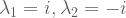
The sum of eigenvalues equals the trace (sum of values along the diagonal).
The product of eigenvalues equals the determinant.

To solve, subtract $\lambda \vec{x}$ from both sides:

$A\vec{x} = \lambda \vec{x}$

$(A - \lambda I)\vec{x} = 0$

We would like to identify n unique eigenvectors. But if the new matrix $(A - \lambda I)$ has an empty nullspace, it will contain zero eigenvectors. So we desire this new matrix to be singular.

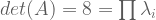
How to accomplish this? By finding eigenvalues that satisfy the characteristic equation $\det(A - \lambda I) = 0$ . Matrices are singular iff their determinants equal zero.

Let’s work through an example! What is the eigendecompositon for matrix $A$ :

$A = \begin{bmatrix} 3 & 1 \\ 1 & 3 \\ \end{bmatrix}$

We need to find eigenvalues that solve the characteristic equation.

$\det(A - \lambda I) = \begin{vmatrix} 3-\lambda & 1 \\ 1 & 3-\lambda \\ \end{vmatrix} = 0$

$(3 - \lambda)^2 - 1^2 = \lambda_2 -6\lambda + 8 = (\lambda-2)(\lambda-4) = 0$

$\lambda_1 = 2, \lambda_2 = 4$

Are these eigenvalues correct? Let’s check our work:

$trace(A) = 6 = \sum{\lambda_i}$

$det(A) = 8 = \prod{\lambda_i}$

How to find our eigenvectors? By solving the nullspace given each eigenvalue.

For $\lambda_1=2$ :

$A - 2I = \begin{bmatrix} 1 & 1 \\ 1 & 1 \\ \end{bmatrix} \Rightarrow rref(A - 2I) = \begin{bmatrix} 1 & 1 \\ 0 & 0 \\ \end{bmatrix}$

$(\lambda_1, \vec{x}_1) = (2, \begin{bmatrix} 1 \\ -1 \\ \end{bmatrix})$

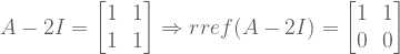
For $\lambda_2=4$ :

$A - 4I = \begin{bmatrix} -1 & 1 \\ 1 & -1 \\ \end{bmatrix} \Rightarrow rref(A - 4I) = \begin{bmatrix} -1 & 1 \\ 0 & 0 \\ \end{bmatrix}$

$(\lambda_2, \vec{x}_2) = (4, \begin{bmatrix} 1 \\ 1 \\ \end{bmatrix})$

Desirable Matrix Properties

The above example was fairly straightforward. But eigendecomposition can “go awry”, as we shall see. Consider a rotation matrix, which in two dimensions has the following form:

$R = \begin{bmatrix} \cos(\theta) & -\sin(\theta) \\ \sin(\theta) & \cos(\theta) \\ \end{bmatrix}$

What are the eigenvalues for rotation $\theta = 90^{\circ}$ ?

$R = \begin{bmatrix} 0 & -1 \\ 1 & 0 \\ \end{bmatrix}$

$\det(R - \lambda I) = \begin{bmatrix} - \lambda & -1 \\ 1 & - \lambda \\ \end{bmatrix} = 0$

$(- \lambda)^2 - 1^2 \Rightarrow \lambda^2 = 1$

$\lambda_1 = i, \lambda_2 = -i$

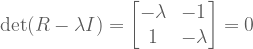
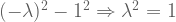
We can check our work:

$trace(R) = 0 = \sum{\lambda_i}$

$det(R) = 1 = \prod{\lambda_i}$

We saw earlier that rotation matrices have no geometric interpretation. Here, we have algebraically shown that its eigenvalues are complex.

$A = \left[ \begin{smallmatrix} 3 & 1 \\ 1 & 3 \\ \end{smallmatrix} \right]$ has real eigenvalues, but $R = \left[ \begin{smallmatrix} 0 & -1 \\ 1 & 0 \\ \end{smallmatrix} \right]$ has less-desirable complex eigenvalues.

We can generalize the distinction between $A$ and $R$ as follows:

Spectral Theorem. Any matrix that is symmetric (A = A^T) is guaranteed to have real, nonnegative eigenvalues. The corresponding n eigenvectors are guaranteed to be orthogonal.

In other words, eigendecomposition works best against symmetric matrices.

Eigendecomposition- Spectral Theorem (1)

Diagonalization

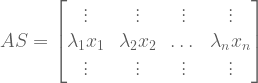
Let us place each eigenvector in the column of a matrix $S$ . What happens when you multiply the original matrix $A$ by this new matrix? Since $S$ contains eigenvectors, multiplication by $A$ reduces to multiplication by the associated eigenvalues:

$AS = \begin{bmatrix} \vdots & \vdots & \vdots & \vdots \\ \lambda_1x_1 & \lambda_2x_2 & \dots & \lambda_nx_n \\ \vdots & \vdots & \vdots & \vdots \\ \end{bmatrix}$

We see the product contains a mixture of eigenvalues and eigenvectors. We can separate these by “pulling out” the eigenvalues into a diagonal matrix. Call this matrix $\Lambda$ (“capital lambda”).

$AS = \begin{bmatrix} \vdots & \vdots & \vdots & \vdots \\ x_1 & x_2 & \dots & x_n \\ \vdots & \vdots & \vdots & \vdots \\ \end{bmatrix} * \begin{bmatrix} \lambda_1 & 0 & \dots & 0 \\ 0 & \lambda_2 & \dots & 0 \\ \vdots & \vdots & \ddots & \vdots \\ 0 & 0 & \dots & \lambda_n \\ \end{bmatrix} = S \Lambda$

Most matrices have the property that its eigenvectors are linearly independent. For such matrices, $S$ is invertible. Given this fact, we can solve for $A$ :

$\Lambda = S^{-1} A S$

$A = S \Lambda S^{-1}$

Matrices that can be factorized in this way are said to be diagonalizable. We can see that both elimination and eigendecomposition are performing the same type of work: factorizing matrices into their component parts.

If $A$ is symmetric, then we know $\Lambda$ is real, and its eigenvectors in $S$ are orthogonal. Let us rename $S$ to be $Q$ , to reflect this additional property. But orthogonal matrices have the property that transposition equats inversion: $Q^T = Q^{-1}$ . Thus, if $A$ is symmetric, we can simplify the diagonalization formula to:

$A = Q \Lambda Q^{-1} = Q \Lambda Q^T$

Asymptoptic Interpretations

This diagonalization approach illustrates an important use case of eigenvectors: power matrices. What happens when $A$ is applied arbitrarily many times? What does the output look like in the limit?

We can use the diagonalization equation to represent $A^k$ :

$A^k = \prod_{i=1}^{k} (Q^{-1} \Lambda Q) = (Q^{-1} \Lambda Q)(Q^{-1} A Q)\dots(Q^{-1} \Lambda Q)$

We can simplify by canceling the inner terms $QQ^{-1}$ :

$A^k = Q^{-1} \Lambda^k Q$

This equation tells us that the eigenvectors is invariant to how many times $A$ is applied. In contrast, eigenvalue matrix $\Lambda$ has important implications for ongoing processes:

If each eigenvalue has magnitude less than one, the output will trend towards zero.
If each eigenvalue has magnitude greater than one, the output will trend to infinity.

Fibonacci Eigenvalues

The powers interpretation of eigenvalues sheds light on the behavior of all linear processes. This includes number sequences such as the Fibonacci numbers, where each number is the sum of the previous two numbers.

Recall the Fibonacci numbers are 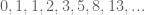$0,1,1,2,3,5,8,13,...$ What is $F_{100}$ ?

Eigenvalues can answer this question. We must first express the Fibonacci generator as a linear equation:

$F(k+2) = 1F(k+1) + 1F(k)$

In order to translate this into a meaningful matrix, we must add a “redundant” equation

$F(k+1) = 1F(k+1) + 0F(k)$

With these equations, we can create a 2×2 Fibonacci matrix $F$ .

$F = \begin{bmatrix} 1 & 1 \\ 1 & 0 \\ \end{bmatrix}$

This matrix uniquely generates Fibonacci numbers.

$u_1 = Fu_0 = \begin{bmatrix} 1 & 1 \\ 1 & 0 \\ \end{bmatrix} \begin{bmatrix} 1 \\ 0 \\ \end{bmatrix} = \begin{bmatrix} 1 \\ 1 \\ \end{bmatrix}$

$u_4 = F^4u_0 = \begin{bmatrix} 1 & 1 \\ 1 & 0 \\ \end{bmatrix}^4 \begin{bmatrix} 1 \\ 0 \\ \end{bmatrix} = \begin{bmatrix} 5 \\ 3 \\ \end{bmatrix}$

To discover the rate at Fibonacci numbers grow, we decompose $F$ into its eigenvalues:

$\det(F - \lambda I) = \begin{vmatrix} 1 - \lambda & 1 \\ 1 & 1- \lambda \\ \end{vmatrix} = 0$

$\lambda^2 - 2\lambda - 1 = 0$

$\lambda_1 = \frac{1 + \sqrt{5}}{2}, \lambda_2 = \frac{1 - \sqrt{5}}{2}$

$\lambda_1 = 1.61803, \lambda_2 = -0.61803$

$trace(F) = 1 = \sum{\lambda_i}$

$det(F) = -1 = \prod{\lambda_i}$

We can go on to discover eigenvectors $x_1$ and $x_2$ . We can then express the Fibonnaci matrix $F$ as

$F = \lambda_1x_1 + \lambda_2 x_2$

$F^k = \lambda_1^k x_1 + \lambda_2^k x_2$

As k goes to infinity, the second term goes to zero. Thus, the ratio is dominated by the larger eigenvalue, 1.61803.

Mathematicians in the audience will recognize this number as the golden ratio.

eigenvectors-fibonacci-and-golden-ratio

We have long known that the ratio of successive Fibonnaci numbers converges to 1.61803. Eigenvalues provide a mechanism to derive this value analytically.

Until next time.

Content Summary: 600 words, 6 min read

And now, an unprovoked foray into number theory!

Simple Continued Fractions (SCFs)

Have you run into simple continued fractions in your mathematical adventures? They look like this:

Let $A$ represent the coefficients $(a_0, a_1, a_2, a_3, ...)$ and $B = ( b_1, b_2, b_3, ...)$ . If you fix $B = (1, 1, 1, ...)$ you can uniquely represent $n$ with $A(n)$ . For example:

$n = \frac{415}{93} = 4+\frac{1}{2+\frac{1}{6+\frac{1}{7}}}$

$A(n) = (4,2,6,7)$

Let us call $A(n)$ the leading coefficients of n. Here we have represented the rational $\frac{415}{93}$ with four coefficients. It turns out that every rational number can be expressed with a finite number of leading coefficients.

Continued Fractions- Number Properties v1

Irrational Numbers

Life gets interesting when you look at the leading coefficients of irrational numbers. Consider the following:

$A(\phi) = (1, 1, 1, 1, 1, 1, 1, ...)$

$A(\sqrt{19}) = (4, 2, 1, 3, 1, 2, 8, 2, 1, 3, 1, 2, 8, ...)$

$A(e) = (2, 1, 2, 1, 1, 4, 1, 1, 6, 1, 1, 8, ...)$

$A(\pi) = (3, 7, 15, 1, 292, 1, 1, 1, 2, 1, 3, 1, ...)$

First note that these irrational numbers have an infinite number of leading coefficients.

What do you notice about $A(\phi)$ ? It repeats, of course! What is the repeating sequence for $A(\sqrt{19})$ ? The sequence $213128$ .

How about $A(e)$ ? Well, after the first two digits, we notice an interesting pattern $211$ then $411$ then $811$ . The value of this triplet is non-periodic, but easy enough to compute. The situation looks even more bleak when you consider the $A(\pi)$ …

Thus $\phi$ (golden ratio) and $\sqrt{19}$ feature repeating coefficients, but $\pi$ and $e$ (Euler’s number) do not. What differentiates these groups?

Of these numbers, only the transcendental numbers fail to exhibit a period. Can this pattern be generalized? Probably. 🙂 There exists an unproved conjecture in number theory, that all infinite, non-periodic leading coefficients with bounded terms are transcendental.

Continued Fractions- Number Properties

Real Approximation As Coefficient Trimming

Stare the digits of $\pi$ . Can you come up with a fraction that approximates it?

Perhaps you have picked up the trick that $\frac{22}{7}$ is surprisingly close:

$\pi = 3.14159265359$

$\dfrac{22}{7} = \textbf{3.14}285714286$

But could you come up with $\frac{22}{7}$ from first principles? More to the point, could you construct a fraction that comes yet closer to $\pi$ ‘s position on the number line?

Decomposing these numbers into continued fractions should betray the answer:

$A(\pi) = (3, 7, 15, 1, 292, 1, 1, 1, 2, 1, 3, 1, ...)$

$A\left(\dfrac{22}{7}\right) = (3, 7)$

We can approximate any irrational number by truncating $A(\pi)$ . Want a more accurate approximation of $\pi$ ? Keep more digits:

$(3, 7, 15, 1) = A(\dfrac{355}{113})$

$\dfrac{355}{113} = \textbf{3.141592}92035$

I’ll note in passing that this style of approximation resembles how algorithms approximate the frequency of signals by discarding smaller eigenvalues.

About π

Much ink has been spilled on the number $\pi$ . For example, does it contain roughly equal frequencies of 3s and 7s? When you generalize this question to any base (not just base 10), the question becomes whether $\pi$ is a normal number. Most mathematicians suspect the answer is Yes, but this remains pure conjecture to-date.

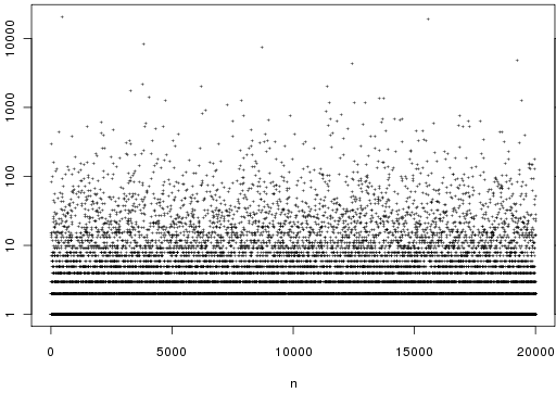
Let’s return to the digits of $A( \pi )$ . Here is a graph of the first two hundred:

Do you see a pattern? I don’t.

Let’s zoom out. This encyclopedia displays the first 20,000 coefficients of $A( \pi )$ :

So $A(\pi)$ affords no obvious pattern. Is there another way to generate the digits of $\pi$ such that a pattern emerges?

Let quadratic continued fraction represent a number $n$ expressed as:

Set $A = (1, 2, 2, 2, 2, ... )$ . Here only $B = ( b_1, b_2, b_3, ...)$ is allowed to vary. Astonishingly, the following fact is true:

$B\left(\dfrac{4}{\pi}\right) = (1, 3, 5, 7, 9, 11, 13, 15, 17... )$

Thus, continued fractions allow us to make sense out of important transcendental numbers like $\pi$ .

I’ll close with a quote:

Continued fractions are, in some ways, more “mathematically natural” representations of a real number than other representations such as decimal representations.

Fewer Lacunae

Distilled, Integrative Research

Tag golden ratio

Eigenvalues and Eigenvectors

Getting Real With Continued Fractions