Part Of: Logic sequence
Followup To: Natural Deduction
Content Summary: 600 words, 6 min read

Motivating Sequent Calculus

Last time, we labelled propositions in the language of verification.

• ↑ represents conjecture: propositions that require verification
• ↓ represents assumption: propositions that can be used for verification.

Two of our connective rules (⊃I and ∨E) expanded our set of assumptions, which we could use at any later time. Logic acumen is invoking the right assumption at the right time.

In contrast to natural deduction, sequent calculus explicitly tracks the set of assumptions) as they vary across different branches of the proof tree.

We will use the turnstile to distinguish assumptions from conjecture: { assumptions } ⊢ { conjectures }

In natural deduction, progress in bidirectional: we are done when we found a connection between assumptions and conjecture. In sequent calculus, progress is unidirectional. Instead, we start with no assumptions, and finish when we have no conjectures left to demonstrate.

Both logical systems rely on two sets of five rules. They bear the following relationships:

• R = I. Right rules are very similar to Introduction rules.
• L = E^-1. Left rules must be turned “upside down”.

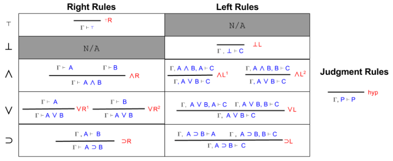
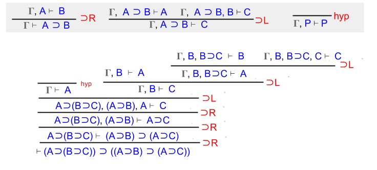
Right and Left rules

We here define capital gamma Γ to represent the context, or current set of assumptions.

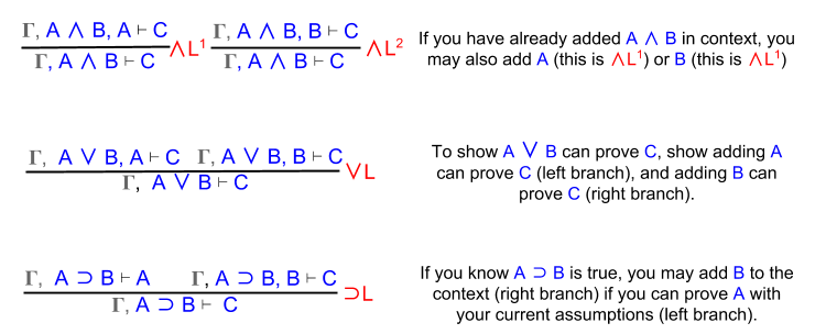
Right rules simply preface Introduction rules with  “Γ ⊢”. The exception ⊃R is instructive. There, A is added to the context, and our “target” conjecture shrinks to just B.

Left rules are less transparently related to Elimination. They are more easily understood by an English explanation:

The entire structure of sequent calculus, then, looks like this:

Enough theory! Let’s use sequent calculus to prove stuff.

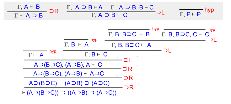
Example 1: Implication

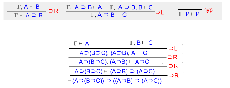
Show that (A ⊃ (B ⊃ C)) ⊃ ((A ⊃ B) ⊃ (B ⊃ C)).

Here, ⊃R serves us well:

We have parsed the jungle of connectives, and arrived at a clear goal. We need to prove C. How?

Recall what ⊃L means: “if you have assumed A ⊃ B, you may also assume B (right branch) if you can prove A with your current assumptions (left branch).

Let’s apply ⊃L to the A ⊃ B proposition sitting in our context. To save space, let us here define Γ with the following three elements: { A⊃(B⊃C), A⊃B, and A }.

We can solve the left branch immediately. Since A ∈ Γ, we can invoke the hyp rule.

Unfortunately, assuming B is not enough to prove C. We must invoke ⊃L again, this time against our A⊃(B⊃C) assumption.

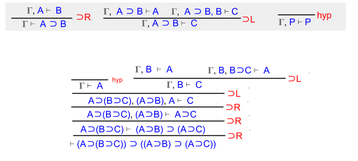
And again, on our newfound B⊃C assumption.

Wait! By now our context by now contains A, B, and C. Each leaf of the proof tree is provable by hyp.

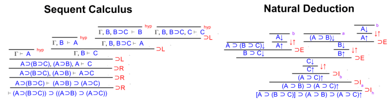
QED. It is instructive to compare this sequent calculus proof with the analogous natural deduction (which we solved together, last time).

Example 2: Distributivity

Show that (A ∨ (B ∧ C)) ⊃ ((A ∨ B)  ∧ (A ∨ C)).

The first two steps here are straightforward. Simplify the conjecture string!

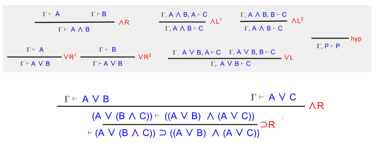
Note that Γ = { A ∨ (B ∧ C) }. Here, we use ∨L to split this assumption into two components:

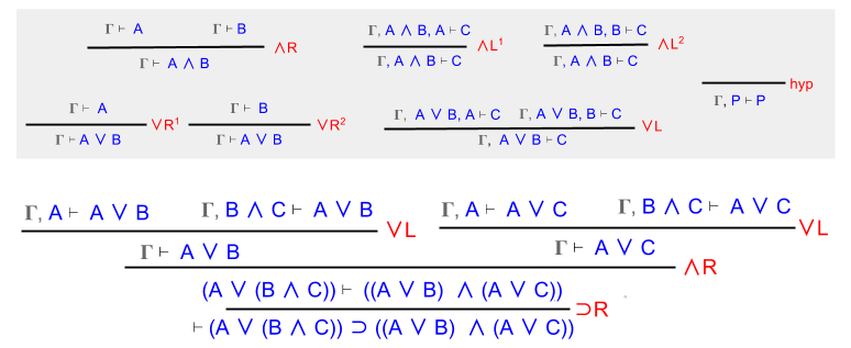
We now have four conjectures to prove. Fortunately, each proof has become trivial:

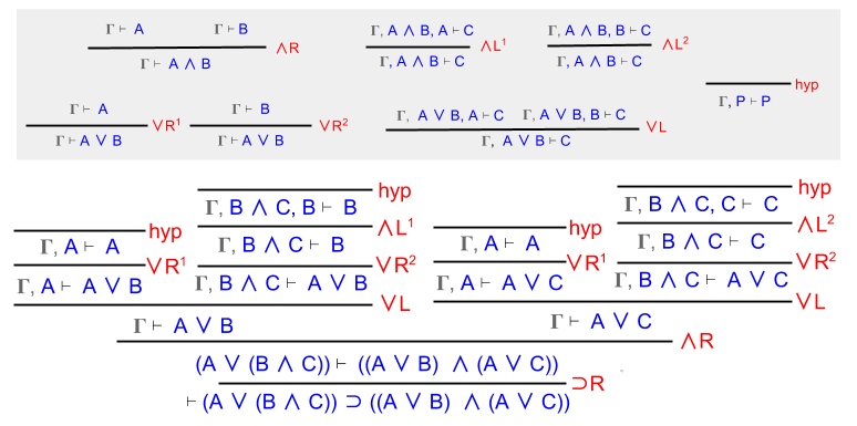
QED.

Takeaways

In this post, we introduced sequent calculus (SC) as an alternative deductive calculus. Sequent calculus makes the notion of context (assumption set) explicit: which tends to make its proofs bulkier but more linear than the natural deduction (ND) style. The two approaches share several symmetries: SC right rules correspond fairly rigidly to ND introduction rules, for example.

If you want to learn sequent calculus for yourself, I recommend solving the converse problems to the two examples above. Specifically,

• Given (A ⊃ B) ⊃ (B ⊃ C), show that A ⊃ (B ⊃ C).
• Given (A ∨ B) ∧ (A ∨ C), show  that A ∨ (B ∧ C).

Until next time!