[Sequence] Game Theory

June 26, 2015January 17, 2019kevinbinz Leave a comment

Main Sequence:

Decision Theory extensions:

An Introduction to Newcomb’s Paradox

Final Report for UW Applied Algorithms class

Computational Trinitarianism

June 26, 2015March 28, 2017kevinbinz 1 Comment

Part Of: Computational Trinitarianism sequence
Content Summary: 1400 words, 14 min read

Ephemeral Proofs

You will be hard pressed to find a mathematician who affirms a theorem without proof. Indeed, mathematical texts are conscientious in pairing mathematical theorem with their proofs.

The tree-like nature of mathematics contributes to its beauty: theorems build on prior results. Theorems are permanent fixtures, solemnly passed from generation to generation.

But what of the proofs? After they convince their audience, they sort of… disappear. Bookmark this sense of confusion; we will return to it in a little while.

What Does Logic Mean?

Consider some proposition A. Most mathematicians would evaluate claims about A as follows:

[A true] means “A is objectively true”
[¬A true] means “A is objectively false”

This ontological interpretation of logic holds that logic encodes facts out there in the world.

But there is also an epistemic interpretation of logic. Consider what it means to interpret propositions as a reflection of our knowledge:

[A true] means “I have a proof of A”
[¬A true] means “I have a refutation of A”

This alternative interpretation of logic is also known as the BHK Interpretation.

Motivating Realizability

The above two interpretations of logic usually coexist fairly peacefully. But in one particular procedure, their differences make themselves known: proof by contradiction. The game goes like this:

Conjecture: A is true.
Proof: Suppose A is false. After exploring this possibility, an absurdity appears. Therefore, A is true.

Let’s get concrete. Here’s an example:

Conjecture: There exists some non-rational numbers a and b such that a^b is rational.

Proof: Suppose there are not two non-rational numbers such that a^b is rational. Consider two examples:

Case A. { a = √2 , b = √2 }.
Case B: { a = √2^√2 , b = √2 }.

It is a fact that √2 is irrational. So Case A contains two non-rational numbers. From our hypothesis we thus know that the output of case A, √2^√2 cannot be rational.

But if √2^√2 is non-rational, then Case B contains two non-rational numbers, and its output must also be non-rational. But:

a^b = (√2^√2)^√2 = √2^(√2*√2) = √2^2 = 2

To say that 2 is non-rational is a contradiction. Therefore, the conjecture is proven.

Classical mathematics is perfectly content with this inference, that ¬¬A = A. But constructive mathematicians would complain that refuting ¬A is not the same as producing a proof of A. It takes considerable effort to show that prove A directly: to prove the non-rationality of some number, you must demonstrate bounds between it and every rational number at some margin.

This is why constructive mathematicians reject the principle of excluded middle, ¬¬A = A as incompatible with their epistemic view of logic. They argue that proof by contradiction desecrates the meaning of the existential quantifier. As Weyl put it in 1946, you have merely “informed the world that a treasure exists without disclosing its location”.

With the BHK Interpretation then, existence is constructive: whenever we claim an object exists, we must provide a way to construct it. This notion is known as realizability, and rejection of excluded middle is known as intuitionism.

The Birth Of Computer Science

It was later found that most of mathematics could be recovered using constructive principles. For example, there does exist a constructive proof that √2^√2 is non-rational. For decades, there was little real progress (or even interaction) between these competing schools. We need to turn to a different field to understand what happens next.

In 1928, David Hilbert challenged the world to provide a procedure that could answer any statement of first-order logic and answer “Yes” or “No”. This “decision problem” (in German, “Entscheidungsproblem“), in many ways prompted the invention of computer science. Hilbert’s problem was solved not once, but three times:

In 1933, Kurt Godel wrote about General Recursive Functions.
In 1936, Alonzo Church introduced his Simply Typed Lambda Calculus
In 1936, Alan Turing invented his eponymous Machine

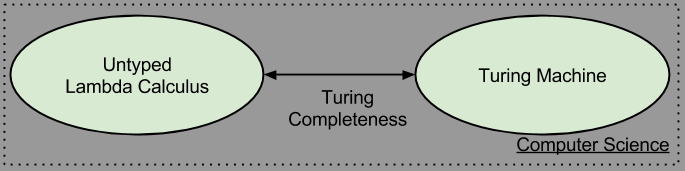
Perhaps dissatisfied with his late submission, Turing went on to show that these wildly divergent systems are, at some deep level, equivalent (“Turing complete”). This is a surprising result.

Computer science did not leverage the above three systems equally, despite their equivalence. Possibly due to its hardware-like aesthetic, the Turing Machine was the conceptual fuel that spawned computer architectures, on which programming languages were designed. But lately lambda calculus, with its “software-first” aesthetic, experienced a major revival. Functional programming languages are based on Church’s system.

While General Recursive Functions are not viewed as particularly implementation-friendly, it is fair to say that the remaining two systems comprise the core of what is computer science:

Trinitarianism- Computer Science Core

bi-CCCs and the Curry-Howard Correspondence

So far, I have been weaving two separate stories: logical interpretation and history of computer science. Haskell Curry is the person who binds my narrative together. In 1958, he began noticing odd similarities between intuitionistic propositional logic (IPL) and the simply typed lambda calculus (STLC). Let me motivate one such similarity here. Both formal systems have operations that do work:

In IPL it is useful to talk about implication (A → B). Implication is useful for encoding sentences like “If Socrates is a man, then he is mortal”.
In STLC, it is useful to talk about “moving inside” a function; the moment when you inject the value of an argument into the content of a function. This operation is known as beta reduction.

These two operations were designed by specialists in different fields, with different motivations, notations, and style of exposition. Nevertheless, if you abstract away all of these all-too-human factors, and stare directly at the underlying formal systems, they begin to smell alike.

The “similar smell” was detected by Haskell Curry in the 1950s and William Howard in the 1960s. As the number of these correspondences increased, the ties between STLC and APL became known as the Curry-Howard Correspondence.

In the 1970s, Joachim Lambek used category theory to provide a fully formal account of this correspondence. It turns out that implication and beta reduction both share the same mathematical structure, and the shape of its construction is named the exponential.

The exponential is not the only shape shared between IPL and STLC. Other equivalences are now understood:

Terminal object & Product
Initial object & Coproduct
Exponential

Formal systems that contain all five of these “shapes” are known as a bi-Cartesian Closed Category (bi-CCC)

Mathematics Is Computation

Don’t fully understand the above section? Good. Each of these equivalences should not “click” without an exploration of how STLC and IPL are implemented. That will come in due time. For now, I ask that you imagine a world in which the Curry-Howard Correspondence is true.

The Correspondence provides a bridge between mathematics and computation.

Computational Trinitarianism

This bridge is very powerful. I opened this post complaining about the second-rate status of proofs in classical mathematics. But our bridge facilitates the following identification: Proofs are programs.

Let me repeat that! A mathematical proof is the exact same thing as a program. Every constructive proof ever created by a mathematician can be made into an algorithm. And every algorithm conceived by a software engineer is ultimately a proof of a mathematical fact.

In logic, proofs are employed as witness to the truth of theorems. Theorems are types. Type theory has been called the Grand Unified Theory of programming languages. The Curry-Howard correspondence provides us with a deep insight: just as a theorems motivate the shape of a proof, types specify the shape of its executing function.

Robert Harper coined the term computational trinitarianism to denote this inter-referential characteristic of type theory, proof theory, and category theory.

You don’t know what you’re talking about, until you understand the idea in all three theories. Once you have all three meanings, you have a genuine scientific discovery. It is permanent.

Takeaways

There are two ways to interpret logic: as a description of the world, or a description of our knowledge
- The latter epistemic view of logic is known as the BHK interpretation
The epistemic view of logic rejects excluded middle and holds that construction precedes existence claims.
- This view of mathematical existence is known as realizability.
Two inventions spawned computer science: the Turing Machine and the Simply Typed Lambda Calculus (STLC)
STLC turns out to be equivalent to intuitionistic propositional logic!
- This “bridge” is named the Curry-Howard Correspondence.
- Category Theory crystallized the shape of the bridge as bi-Cartesian Closed Categories.
The Curry-Howard Correspondence unifies mathematics and computation
- Proofs are Programs, and Theorems are Types
- Any mathematical proof can be translated into a program, and vice versa.

Nash Equilibria

June 7, 2015March 22, 2017kevinbinz Leave a comment

Followup To: An Introduction To Prisoner’s Dilemma
Part Of: Algorithmic Game Theory sequence
Content Summary: 500 words, 5 min read

Consider the following game:

Both spouses prefer the company of one another. In fact, they spent the evening together, they incur zero cost. However, if faced with a choice of waiting in an empty house vs. earning some overtime, they would prefer the latter twice as much.

We encode this game’s strategy-space as follows:

Recall our previous discussion of Pareto optimality and strategic dominance. There are myriad ways to think about games, why isolate those two properties, in particular? One reason to invent names is to construct a universal toolkit: non-trivial properties that exist in all games, and amenable to our analyses.

Pareto optimality makes an appearance in the above game (H, H). But strategic dominance does not. Take a moment to convince yourself this is true.

Since strategic dominance is too strong to be a universal property, we might relax it. What happens when we encode regret? That is, what does the Spousal Game look like after we consider cases when a player wishes she had made a different choice?

Arrows represent regret.

In bottom-left cell, Spouse A wishes she had worked (purple arrow right) but Spouse B wishes he had gone home (orange arrow up).
In top-right cell, we see an entirely symmetric expression of mutual regret.
In the remaining cells, neither spouse can do better by individually changing their strategy.

Let us view Prisoner’s Dilemma from the same lens.

These arrows have a peculiar pattern. Why? Because of strategic dominance!

We can explain strategic dominance in terms of regret. That is, if a player’s regrets are all in the same direction, then that player is subject to strategic dominance.

Does regret belong in our universal toolbox? No. Regret by itself is rather uninteresting: every game with non-trivial utilities comprises myriad regrets.

We need a stronger property. How about games containing outcomes with no regret? Call such outcomes Nash equilibrium.

Does every game have Nash equilibria?

Prisoner’s Dilemma has one: (D, D)
Spousal Game has two: (H, H) and (W, W)

Perhaps no game fail to have this peculiar creature..

Conjecture 1: Every game with a finite number of players and strategies has at least one Nash equilibrium.

Time to search for counter-examples! Consider the game Rock-Paper-Scissors. Here’s how it looks to a game theorist:

Crucially, every node has at least one arrow leaving it. Rock/Paper/Scissors has no equilibrium! We have thus disproven Conjecture 1. What now?

In addition to the absence of Nash equilibria, this game is interesting in another sense. It turns out that having a deterministic strategy in Rock/Paper/Scissors is a bad idea. In fact, machines can reliable beat people at Rock/Paper/Scissors by exploiting patterns in human gameplay.

What happens when we expand our notion of game to incorporate non-deterministic strategies. The best mixed strategy a player can adopt is [⅓ ⅓ ⅓]; that is where each choice is randomly selected with probability 0.33.

While hard to visualize, it is easy to intuitively grasp the existence of a new equilibrium. If each player adopts [⅓ ⅓ ⅓], neither will experience regret! Thus we can safely repair our Conjecture:

Conjecture 2. Every game with a finite number of players and strategies has at least one Nash equilibrium if mixed strategies are allowed.

It turns out that Conjecture 2 is entirely correct. In fact, its correctness is one of the most significant results in all of game theory.

An Introduction To Prisoner’s Dilemma

June 5, 2015March 22, 2017kevinbinz Leave a comment

Part Of: Algorithmic Game Theory sequence
Content Summary: 600 words, 6 min read

Setting The Stage

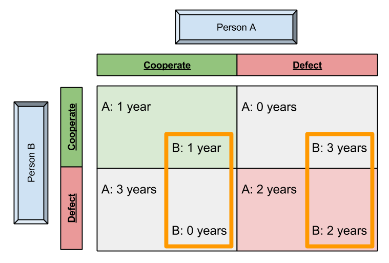
The Prisoner’s Dilemma is a thought experiment central to game theory. It goes like this:

Two members of a criminal gang are arrested and imprisoned. Each prisoner is in solitary confinement with no means of speaking to or exchanging messages with the other. The police admit they don’t have enough evidence to convict the pair on the principal charge. They plan to sentence both to a year in prison on a lesser charge.

Simultaneously, the police offer each prisoner a Faustian bargain. Each prisoner is given the opportunity either to betray the other, by testifying that the other committed the crime, or to cooperate with the other by remaining silent:

If A and B both betray the other, each of them serves 2 years in prison

If A betrays B but B remains silent, A will be set free and B will serve 3 years in prison (and vice versa)

If A and B both remain silent, both of them will only serve 1 year in prison (on the lesser charge)

Do you “get” the dilemma? Both prisoners do better if they each cooperate with one another. But they are taken to separate rooms, where the decisions of the other are no longer visible. The question evolving towards one of trust…

This parable can be drawn in strategy-space:

Strategic Dominance

Consider Person A’s perspective:

One line of analysis might run as follows:

If the other person cooperates (top rectangle), Player A would do better defecting (rightmost cell).
If the other person defects (bottom rectangle), Player A would do better defecting (rightmost cell).

Thus, no matter what B’s choice, defection leads to a superior result. Let us call this strategic dominance.

Person B’s perspective, in the below figure, is analogous:

If the other person cooperates (left rectangle), Player A would do better defecting (bottom cell).
If the other person defects (right rectangle), Player A would do better defecting (bottom cell).

Thus, the strategically dominant outcome is Defect-Defect, or (D, D).

Pareto Optimality

If the prisoners could coordinate their responses, would they select (D,D)? Surely not.

How might we express our distaste for mutual defection rigorously? One option would be to notice that (C, C) is preferred by both players. Is there anything better than mutual cooperation, in this sense? No.

Let us call the movement from (D,D) to (C,C) a Pareto improvement, and the outcome (C,C) Pareto optimal (that is, no one player’s utility can be improved without harming that of another).

It turns out that (C,D) and (D, C) are also Pareto optimal. If we map all outcomes in utility-space, we notice that Pareto optimal outcomes comprise a “fence” (also called a Pareto frontier).

The crisis of the Prisoner’s Dilemma can be put as follows: (D, D) doesn’t reside on the Pareto frontier. More generally: strategically-dominant outcomes need not reside on the Pareto frontier.

While there are other, more granular, ways to express “good outcomes”, the Pareto frontier is a useful way to think about the utility landscape.

Let me close with an observation I wish I had encountered sooner: utility-space does not exist a priori. It is an artifact of causal processes. One might even question the ethics of artificially inducing “Prisoner’s Dilemma” landscapes, given their penchant for provoking antisocial behaviors.

Takeaways

A strategy is called dominant when it always outperforms alternatives, irrespective of competitor behavior.
Pareto optimal outcomes are those for which there is no “pain-free” way to improve the outcome of any participant. All such outcomes comprise the Pareto frontier.
The Prisoner’s Dilemma illustrates that strategically-dominant outcomes need not reside on the Pareto frontier, or more informally, that acting in one’s self-interest can lead to situations where everyone loses.

Getting Real With Continued Fractions

April 29, 2015March 23, 2017kevinbinz Leave a comment

Content Summary: 600 words, 6 min read

And now, an unprovoked foray into number theory!

Simple Continued Fractions (SCFs)

Have you run into simple continued fractions in your mathematical adventures? They look like this:

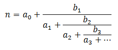
Let $A$ represent the coefficients $(a_0, a_1, a_2, a_3, ...)$ and $B = ( b_1, b_2, b_3, ...)$ . If you fix $B = (1, 1, 1, ...)$ you can uniquely represent $n$ with $A(n)$ . For example:

$n = \frac{415}{93} = 4+\frac{1}{2+\frac{1}{6+\frac{1}{7}}}$

$A(n) = (4,2,6,7)$

Let us call $A(n)$ the leading coefficients of n. Here we have represented the rational $\frac{415}{93}$ with four coefficients. It turns out that every rational number can be expressed with a finite number of leading coefficients.

Continued Fractions- Number Properties v1

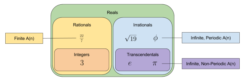
Irrational Numbers

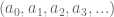
Life gets interesting when you look at the leading coefficients of irrational numbers. Consider the following:

$A(\phi) = (1, 1, 1, 1, 1, 1, 1, ...)$

$A(\sqrt{19}) = (4, 2, 1, 3, 1, 2, 8, 2, 1, 3, 1, 2, 8, ...)$

$A(e) = (2, 1, 2, 1, 1, 4, 1, 1, 6, 1, 1, 8, ...)$

$A(\pi) = (3, 7, 15, 1, 292, 1, 1, 1, 2, 1, 3, 1, ...)$

First note that these irrational numbers have an infinite number of leading coefficients.

What do you notice about $A(\phi)$ ? It repeats, of course! What is the repeating sequence for $A(\sqrt{19})$ ? The sequence $213128$ .

How about $A(e)$ ? Well, after the first two digits, we notice an interesting pattern $211$ then $411$ then $811$ . The value of this triplet is non-periodic, but easy enough to compute. The situation looks even more bleak when you consider the $A(\pi)$ …

Thus $\phi$ (golden ratio) and $\sqrt{19}$ feature repeating coefficients, but $\pi$ and $e$ (Euler’s number) do not. What differentiates these groups?

Of these numbers, only the transcendental numbers fail to exhibit a period. Can this pattern be generalized? Probably. 🙂 There exists an unproved conjecture in number theory, that all infinite, non-periodic leading coefficients with bounded terms are transcendental.

Continued Fractions- Number Properties

Real Approximation As Coefficient Trimming

Stare the digits of $\pi$ . Can you come up with a fraction that approximates it?

Perhaps you have picked up the trick that $\frac{22}{7}$ is surprisingly close:

$\pi = 3.14159265359$

$\dfrac{22}{7} = \textbf{3.14}285714286$

But could you come up with $\frac{22}{7}$ from first principles? More to the point, could you construct a fraction that comes yet closer to $\pi$ ‘s position on the number line?

Decomposing these numbers into continued fractions should betray the answer:

$A(\pi) = (3, 7, 15, 1, 292, 1, 1, 1, 2, 1, 3, 1, ...)$

$A\left(\dfrac{22}{7}\right) = (3, 7)$

We can approximate any irrational number by truncating $A(\pi)$ . Want a more accurate approximation of $\pi$ ? Keep more digits:

$(3, 7, 15, 1) = A(\dfrac{355}{113})$

$\dfrac{355}{113} = \textbf{3.141592}92035$

I’ll note in passing that this style of approximation resembles how algorithms approximate the frequency of signals by discarding smaller eigenvalues.

About π

Much ink has been spilled on the number $\pi$ . For example, does it contain roughly equal frequencies of 3s and 7s? When you generalize this question to any base (not just base 10), the question becomes whether $\pi$ is a normal number. Most mathematicians suspect the answer is Yes, but this remains pure conjecture to-date.

Let’s return to the digits of $A( \pi )$ . Here is a graph of the first two hundred:

Do you see a pattern? I don’t.

Let’s zoom out. This encyclopedia displays the first 20,000 coefficients of $A( \pi )$ :

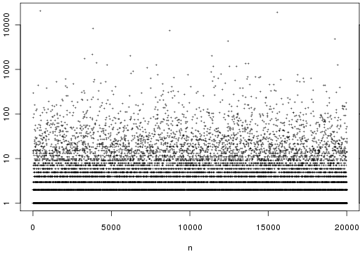
So $A(\pi)$ affords no obvious pattern. Is there another way to generate the digits of $\pi$ such that a pattern emerges?

Let quadratic continued fraction represent a number $n$ expressed as:

Set $A = (1, 2, 2, 2, 2, ... )$ . Here only $B = ( b_1, b_2, b_3, ...)$ is allowed to vary. Astonishingly, the following fact is true:

$B\left(\dfrac{4}{\pi}\right) = (1, 3, 5, 7, 9, 11, 13, 15, 17... )$

Thus, continued fractions allow us to make sense out of important transcendental numbers like $\pi$ .

I’ll close with a quote:

Continued fractions are, in some ways, more “mathematically natural” representations of a real number than other representations such as decimal representations.

Bridging the Is-Ought Gap

April 2, 2015April 7, 2017kevinbinz Leave a comment

Part Of: Demystifying Ethics sequence
Prerequisite: An Introduction to Propriety Frames
Content Summary: 1400 words, 14 min read

Introduction

This article presents a theory of normatives. It is not a complete theory (it does not even describe implementation), nor does it answer a number of important objections. I sketch it, in its current state, in order to motivate the claim that explaining normatives is possible.

Hyperpoints

Consider again the problem of describing locations in a space. In a two dimensional space, any coordinate system I use (e.g., Cartesian or polar) require two pieces of data to uniquely specify the location. In a space with three degrees of freedom, three points of data are required. Call this symmetry between dimensionality and data the data-dimension bridge.

Your brain is embedded in a three dimensional space, and your visual system evolved in this context. It is just as mathematically meaningful to discuss locations in a 17D space, despite the fact that you lack the mental equipment to visualize it.

Take this argument to an extreme. The universe contains approximately 10^82 atoms. If we suppose there are 100 interesting facts we can name for every atom, this means that we need 10^84 data points to describe the universe. Given our data-dimension bridge, this means that the entire universe can be described by the location of one point in a (10^84)D space.

Such hyperpoints turn out to be a surprisingly versatile concept, appealed to frequently by mathematicians. They were first introduced in an inaugural lecture by Bernhard Riemann in 1854.

Propriety Frames

Main Article: An Introduction To Propriety Frames

Our everyday lives are immersed in highly structured interactions. Much of these community expectations are taken for granted; they are practically invisible to us. But if you travel to a culture sufficiently remote from your own, or spend much time around people suffering from Asperger’s syndrome, and you can begin to build an appreciation for these culturally-approved roles.

Consider a typical evening spent at a fancy restaurant. If I asked you to come up with a complete list of examples of things that would surprise you, how long do you think that list would be? Consider some representative examples.

The waiter states he is not in the mood to take your order.
Several guests are engaged in a foodfight.
An expensive item on the menu is marked as free of charge.
Instead of payment, the manager comes out to request that you wait tables next weekend.
The food is dumped directly on the table.
On taking a bite, you realize that your meal is actually plastic: an artistic creation designed purely for visual effect.

The length of the list corresponds to the volume of knowledge embedded within your brain’s social intuitions.

Social psychology likes to speak of frames as a useful way to bundle collections of facts together. We can say that our restaurant experience is defined as the intersection of three different frames: host-guest, place of business, eating. Each of the above surprises are produced by a violation of one of these frames.

Propriety Frames- Restaurant Example (3)

When a mother instructs her son to not yell in the store, the child installs an update to his Shopping frame. When a family exchanges gossip around a campfire, they are doing so in part to synchronize their propriety frames.

Mental Hyperpoints

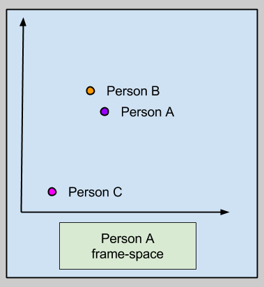
Time to synthesize the above. Each social frame can be decomposed into a collection of facts. Thus, a person’s social intelligence can be fully described by a hyperpoint in frame-space.

In fact, we can represent any mental process in terms of hyperpoints. In the following graphic, we are representing the social memory, semantic memory, and perceptual memory.

Take a moment to appreciate this graphic. Every sentence you utter, every subtlety of your body language, every friendship you have ever formed: the totality of your life as an organism is captured as a single point in behavior-space.

Did you notice how Person A only encodes other people in behavior-space? This is because human beings do not have direct access to one another’s mental lives. That said, we can imagine that knowledge of another person’s behavior may let us estimate the social rules they hold as legitimate.

A Theory Of Normatives

Let’s switch gears. What does it mean for somebody to say “you should buy this stock” or “you should not blackmail your coworkers”?

We call statements with “should” in them normative language. These contrast with descriptive statements of reality. David Hume noticed this distinction clearly, and formulated what is now known as the is-ought gap:

In every system of morality, which I have hitherto met with, I have always remarked, that the author proceeds for some time in the ordinary ways of reasoning, and establishes the being of a God, or makes observations concerning human affairs; when all of a sudden I am surprised to find, that instead of the usual copulations of propositions, is, and is not, I meet with no proposition that is not connected with an ought, or an ought not. This change is imperceptible; but is however, of the last consequence. For as this ought, or ought not, expresses some new relation or affirmation, ’tis necessary that it should be observed and explained; and at the same time that a reason should be given, for what seems altogether inconceivable, how this new relation can be a deduction from others, which are entirely different from it.

With this backdrop, I would like to propose the following three-part theory of normatives.

First, normatives are nothing more than hyperpoints in frame-space, tagged by a separate module with a “should” label. Call these marked hyperpoints normative attractors. As evidence, consider that every statement of “ought” can be cast back into descriptive language (“you should do X” can be translated into “good people do X”).

Second, normative attractors are fed into our motivational subsystems. The word “ought” is not just a fun word to throw around, it evolved to promote behavioral change.

Third, normatives co-evolved with natural language. Recall the functional purpose of language: to allow humans to exchange mental information. Mental information about the world (human semantic memory) required no additional hardware to synchronize: perceptual psychophysics provides a sufficient reference point. But coordinating social frames had no such advantage, and required new hardware (the attractor).

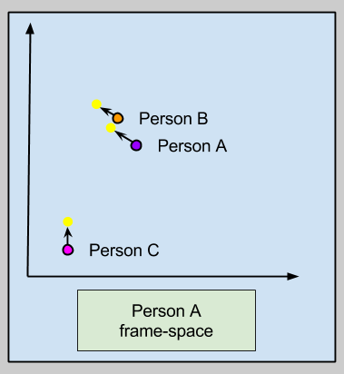
Let us call this toy hypothesis the Frame Attractor theory of normatives. Here’s an illustration; where the yellow attractor represents Person A’s vision of optimal behavior (e.g., Buddha, Jesus, “being nice”, etc):

Disaggregated Attractors

It is a virtue of explanatory models to consume prior considerations under a more comprehensive framework. I have used this model to improve my understanding of why conflicts happen, and how to resolve them peaceably. This is left as an exercise to the reader. 🙂

In the above image, consider the plight of Person C. Is the sheer distance between their behavior and the norm motivating?

In Normative Therapy, I state the following:

Let me zoom in on one “population subset”: the sociopath. Such an individual is biologically incapable of meeting aggregate-level normative impositions such as “everyone should care about the well-being of those around them”. The argument here, is that normative impositions should be explicitly tailored to the individual situation; for people like sociopaths, this would be something like, “sociopath X should put herself in situations where her non-empathic behavior can be held accountable”.

This observation, and the argument underlying that post, suggests that it may be advisable to disaggregate normatives. If the goal of morality to more effectively move people towards the normative attractor, perhaps innovation in cultural technology will permit stable individuated attractors, like this:

The above example uses disaggregated normatives as lures to attract people towards The Goal. But this is not the only use of such a mechanism. Perhaps we could also train personal-attractors in a more diverse ethical setting with multiple Goals. But, for now, let me leave such a question for another day.

Takeaways

Thinking about complex ideas as locations in a high-dimensional space (hyperpoints) is a surprisingly powerful conceptual tool.
Complex community rules are most likely implemented via a particular memory system that encodes social frames.
The Frame Attractor theory of normatives is grounded in three principles
1. “Ought language” are hyperpoints in frame-space, tagged with a “should” label. Call these normative attractors.
2. Normative attractors are fed into our motivational subsystems.
3. Normatives co-evolved with natural language.
This theory can be used to explain other arguments, such as my argument in support of person-specific normatives.

The Psychology Of Chess

March 29, 2015June 27, 2017kevinbinz 1 Comment

Part Of: Chess sequence
Followup To: The Chess SuperTree
Content Summary: 1400 words, 14 min read

Dual Process Cognition: Working Memory

Chess engines operate by generating a decision tree, pruning irrelevant branches, assigning scores to the leaves, and consulting the minimax oracle for an optimal decision.

But when we switch from silicon to grey matter, we notice that the human mind is structured differently. We can be meaningfully divided into two selves: a fast, autonomic, associative mind and a slow, serial, conscious mind. What’s worse, the content of our “more rational” self is small – System II is grounded in working memory, which can hold 7 +/- 2 chunks of information.

Working memory span is highly correlated with IQ. Keith Stanovich, in his Rationality and the Reflective Mind, claims that intelligence can be understood as a cognitive decoupling; that is, highly intelligent people are able to evaluate more hypothetical scenarios faster, and keep those explorations firewalled from one’s modeling of the current reality.

While playing chess, the ability to construct a decision tree is a conscious, effortful task. In other words, decision trees are instantiated within your System II working memory during game play.

Dual Process Cognition: Somatic Markers

If decision trees are consciously maintained, what is the basis of score evaluation functions? Recall that machine learning accomplishes this by virtue of training feature vectors and weight vectors. Suppose these vectors can contain two millions numbers each. Every time the engine is asked to evaluate a position, it will compute a dot product: scan over the vectors, and for each value record its product.

With decision trees, I can remember keeping various alternatives in my head. Not so with producing decision scores. Nothing in my gameplay experience feels like I am computing two million numbers with every move. This suggests that score evaluation functions happen within the subconscious, massively parallel System I.

But what does evaluating a position feel like? Two phenomenological observations are in order:

Playing chess is a highly intuitive, emotional affair. Positions in which we have a strong advantage feel good, moves that lead us into checkmate feel scary, and the objectively optimal move tends to produce the most positive feeling. In other words, emotion is the mediator of chess skill. This is an expression of the somatic marker hypothesis.
Explaining chess moves tends to naturally flow in a non-mathematical language, where reasons are considered the final authority over decision making. I am better able to remember “White is better because he has an attack” instead of “White is 20% more likely to win the game”.

We’ll return to these suggestive observations in a little bit.

Is Scoring Cardinal Or Ordinal?

In economic theory, all decisions are mediated by a psychological entity called utility. (I introduce this concept in this post). Neuroeconomics is an attempted integration between economics, psychology, and neuroscience; it tries to get at how the brain produces decisions. Within this field, there is a live debate whether the brain represents utility cardinally (e.g., 3.2982) or ordinally (e.g., A > B and B > C).

Consider again how chess engines compute on the decision tree. The minimax algorithm pushes leaf nodes up the tree, merging results via the min() or max() operation. Whereas engines perform these operation against cardinal score nodes (e.g., in fractions of a pawn called centipawns), this need not be the case. Taking the max(A, B) does not require knowing the precise value of A and B. It is sufficient to know that A > B. In other words, minimax can also work against an ordinal scoring scheme.

The implications of an ordinal scoring scheme becomes more apparent if you view the minimax algorithm from a comparison perspective. In the following image, white spheres represent White decisions (maximization) and gray spheres represent Black decisions (minimization).

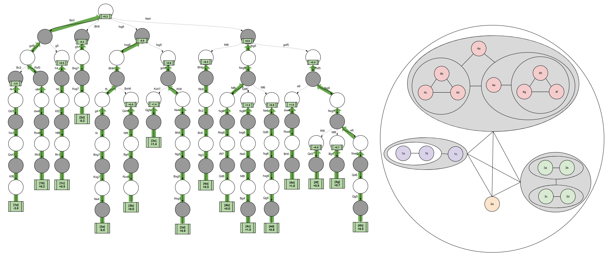
It is possible to think of image on the left as a “side view” of the minimax algorithm. With this geometric interpretation, the right image becomes a “bottom view” of the exact same algorithm. Pause a moment here until you convince yourself of this.

Consider the nested spheres containing the purple nodes. These represent three leftmost threads in the decision tree: { { 1a vs 1b } vs 1c }. Do we need to know the value of { 1a vs 1c } or { 1b vs 1c }? If we knew both facts, we could surely have enough information to implement minimax. But this “easy solution” would require a total ordering, which is prohibitively expensive. We instead need to resolve the { 1a vs 1b } fact, after which we can compare the result to 1c.

So the brain could choose to evaluate positions ordinally or cardinally. Which technology does it employ in practice?

I don’t know, but I can recommend a test to divine the correct answer. The order in which cardinal scores are generated is unconstrained: a chess player with a cardinal function can evaluate any position at any time. In contrast, the order in which ordinal scores are generated is highly constrained (if we assume a non-total ordering). A brain that implement ordinal evaluations cannot physically evaluate the 1c thread until it has evaluated { 1a vs 1b }. Thus, if we were to study the speech and subjective experiences of a multitude of chess players, we could hope to learn whether their creative abilities are constrained in this way.

The State Comparator & Distinguishing Features

Consider again the feature-weight dot product model of score functions. If I were to evaluate two very similar functions, the dot product would necessarily be very similar: only a few dozen features may meaningfully diverge in their contribution to the final output. Call these uniquely divergent features the distinguishing features.

A computer engine will compute similar dot products in their entirety (with the exception of position that are exactly the same, see transposition tables); it strikes me as very likely that the brain (a metabolic conservative) typically only retains a representation of the distinguishing features. In other words, the “reason-based natural language” that humans produce when we evaluating gamelines draws from a cognitive mechanism that recognizes that features close in distance to the KingSafety category tend to be the relevant ones.

In the discussion of Decision Trees In Chess, I discuss four different moves. The insightful reader may have noticed that I moved my Bishop to the h6 square in three separate situations. These considerations happen at three locations in the decision tree:

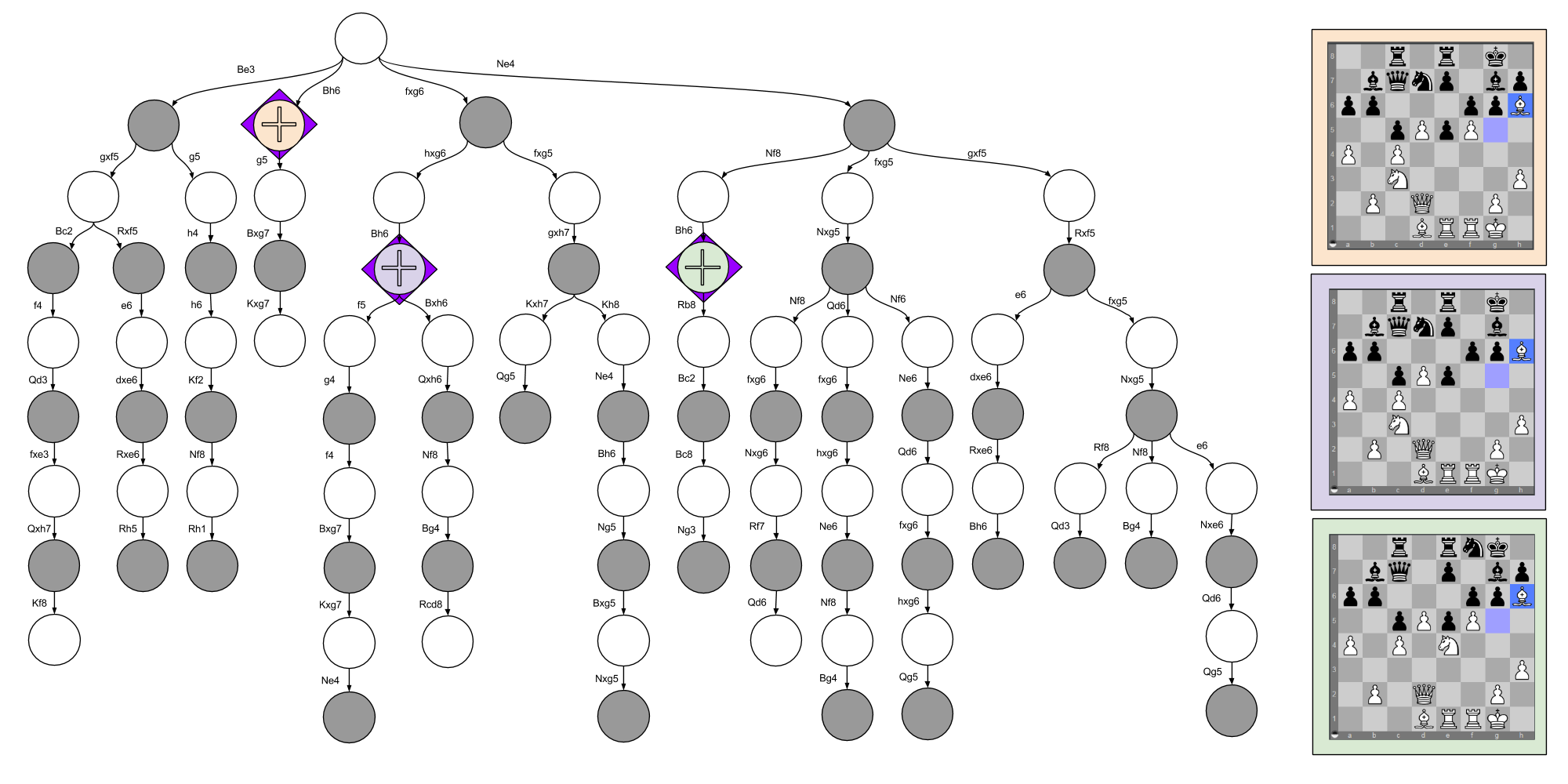
While a chess engine may score each position repetitively, each score computation will be very similar. Only two features really stand out:

The purple node is different from the orange node because the former has traded off two pawns.
The green node is different from the orange node because the former has made two Knight moves to attack & defend the Kingside.

If you consult the minimax graphic above, you’ll see that my preference ordering is { Green > Orange > Purple }. I would explain this in language by appealing to the relevant differences (e.g., “the pawn trade frees his pawns to control the center”). To me, this is evidence for a state comparison tool that is able to zoom in on distinguishing features.

The Move Generator & Representative Lines

Another distinction between human and computer decisions in chess seems to lie in how the decision tree is approached. Engines like Stockfish typically have a getLegalMoves() function that fleshes out the entire branching structure, and then (extremely) sophisticated pruning techniques are used to make truly deep evaluations possible of the interesting lines. It is possible that nonconscious Type I processes in humans do something comparable, but this strikes me as unlikely. Rather than an eliminative approach to the SuperTree, it seems to me that humans construct representations gradually.

Specifically, I suspect that humans have a Type I statistical mechanism that generates a few plausible moves for a given position. Consider the following subset of a decision tree I examined previously:

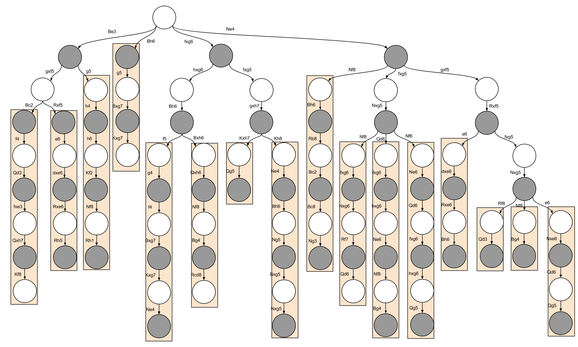
Each orange rectangle represents moments when I simply stopped considering alternatives; these representative lines are depth-oriented in nature. I suspect the ubiquity of these representative lines can be explained by appealing to serial application of the MoveGenerator, and the sheer difficulty humans have in maintaining a complex tree in working memory.

Takeaways

The brain represents decision trees largely in working memory (a conscious System II process)
Massively parallel System I processes are how the brain computes position scores, which are encoded in emotion.
While computers represent scores as numbers, it is possible the brain represents scores as preferences (an ordinal system).
The brain, being allergic to duplicate computations, contains a State Comparator which isolates distinguishing features within similar positions.
Rather than pruning a complete decision tree like computers, the brain an intuitive, System I, Move Generator to construct a plausible sub-tree.

The Chess SuperTree

February 28, 2015June 27, 2017kevinbinz Leave a comment

Part Of: Chess sequence
Followup To: Decision Trees In Chess
Content Summary: 1500 words, 15 min read

Chess Is A Nested Algorithm

In An Introduction To Chess, I introduced you to the basics of chess analysis: how to tell when one position is better than another. Specifically, we looked at material, pawn structure, space, king safety, piece development, piece cohesion, and initiative. These ways of thinking about different chess positions were combined into a score. The first aspect of chess thought lies in the maturation of such an scoring function.

In Decision Trees In Chess, I introduced you to the basics of chess decision making: how to evaluate different alternatives when you are not sure what to do. Specifically, we looked at how imagining different scenarios can be represented in decision trees, how these trees ultimately use scoring functions in their leaf nodes. These decision trees produce decisions after application of the minimax algorithm.

Together, scoring functions and decision trees describe the entirety of what it is to do chess. Had this series been written by world champion Magnus Carlsen, I submit that even he could communicate effectively using this two-part framework. The only things that need be different would be his analysis (his scoring function would be more accurate) and his choice of alternatives to analyze (his considered choices would contain fewer bad alternatives). In other words, skill in chess is not doing more than score functions and decision trees. It is doing them well.

Two Kinds Of Score

Consider the following. White’s turn, can you find mate in two moves?

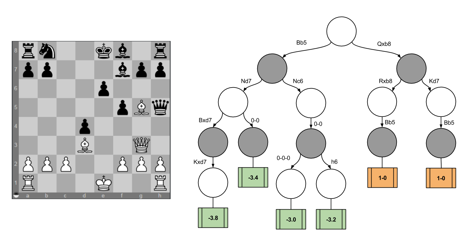
The solution to this puzzle, displayed on the rightmost decision tree, is Qxb8+. If Black recaptures, White checkmates with Bb5# (note that the Bg5 prevents Black’s king from escaping (and if Black runs away Kd7, he is met with the same fate).

Now, imagine if White had not found this clever solution immediately. Suppose White instead tries to attack Black with Bb5+. White’s reflections could lead him to consider the other decision tree, which ultimately values Bb5 as -3.2 points (do you see why the minimax algorithm requires this to be the case?)

Consider the returned values (1-0 WIN) for Qxb8+, and (-3.2) for Bb5. This incongruity is itchy. Why would the scoring function return different types of answers depending on the position?

Meet The SuperTree

Imagine for a moment the decision tree for all chess games. Call this object the SuperTree. What does it look like?

Consider the following facts:

On move zero, all chess games ever begin in the same position.
After white’s first move, all chess games ever are in one of twenty possible positions (White has 20 legal moves)
After Black’s first move, all chess games ever are in one of four hundred possible positions (20*20)
All chess games ever conclude with a result (White wins, Black wins, or tie). Some games finish quickly, others take many moves.

These facts can be consolidated into the following visualization:

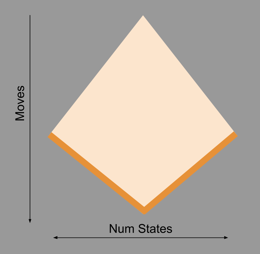
Consider the top of the SuperTree: as we move our gaze downwards, its width increases. This corresponds to our observation above that, as more moves are made, the number of possible positions rapidly increases.

Why then does the number of possible positions decrease as we move into the endgame? Well, you have surely noticed how endgames tend to feature fewer pieces. Consider all chess games that have transitioned into King+Queen vs. King. There are only a few thousand ways to place these three pieces on the board (64*63*62 = 249,984 is an upper bound). Fewer pieces means fewer states (which is why the Supertree is shown as a diamond, not of a triangle).

At the end of every game, at the end of a game tree, are result nodes. This are represented by the dark orange boundary.

We have so far analyzed two game positions: my game from the Decision Trees In Chess post, and the Mate-In-Two position above. Since the above cartoon claims to comprise all chess games that can ever be played, let’s see how these games fit into the SuperTree.

On the left, we see that the Mate-In-Two game line from this post is shorter: this reflects that it (presumably) terminated in the early middlegame, whereas my opponent in the last post survived until the 53rd move.

On the right, we see the decision trees we constructed at moments in each of these games. Pay attention to the coloring of these trees: in the earlier analysis, our endpoints we numerical scores (green) which propagate up to the top of the triangle. In today’s analysis, our endpoints contain a mixture of numerical scores (green) and final results (orange). In this case, by minimax logic, the orange style of result successfully propagated to the top of the decision tree.

Can Chess Be Solved?

Final results, like numerical scores, propagate up a decision tree. If we start at the end of chess games, and work our way backwords, could we color the entire cartoon orange? Could we banish these numerical scores and solve chess? By “solve chess”, I mean be able to prove perfect play; that is, to be able to prove, from any position, the correct move (including move 1).

Lest I be accused of dreaming of something too implausible, precisely this has been done for games like Checkers and Connect-4 (more examples here).

It turns out that chess has been partially solved: computer scientists have managed to solve all games that land in King+Queen vs. King positions. Don’t believe me? Go here, and experience for yourself what it is like to play against God.

We can visualize on our cartoon how computer scientists have managed to “pull orange upwards” in an attempt to solve the SuperTree. These results are typically referred to as tablebases.

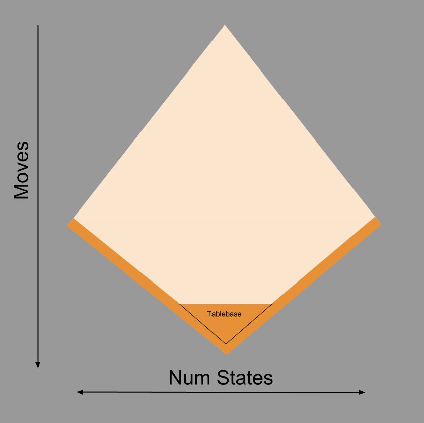
Why haven’t tablebases reached the top of the SuperTree? Compare the size of tablebases as we increase the number of pieces. A three-piece tablebase would include, for example, our classic example of King+Queen vs. King. Such a tablebase only requires 62 kilobytes of memory. But consider what happens when we accomodate more pieces:

Number Of Pieces	Tablebase Size (Bytes)
3	62,000	62 kB
4	30,000,000	30 MB
5	7,100,000,000	7.1 GB
6	1,200,000,000,000	1.2 TB
7	140,000,000,000,000	140 TB

To my knowledge, to date our modern supercomputers have failed to construct a complete 8-piece tablebase. Chess begins with 32 pieces. From the table above, when do you think the human race will possess enough computing resources to implement a 32-piece tablebase? 🙂

A Role For Numeric Scores

We now see why our scoring function cannot return game results for most moves in our path.

Consider the case where the results of the Supertree propagate upwards in a completely unpredictable manner. In this situation, we could do no better than rolling a dice to make our move, because no move can increase or chances of winning (or losing, or drawing).

But chess is not like this. Suppose you convince two evenly-matched players to play 100 games, and you remove the queen from the first player’s starting position before each match begins. The second player will probably win many more than 50 games. This tells us that chess results are not completely unpredictable. Locations in the SuperTree in which one player has a material advantage have an above-average chance of leading to a Win result, just as material disadvantages tend to balance the scale towards the Lose result. Given this window of improved predictability, we can prefer moves that improve our material situation.

Most moves in chess, regrettably, do not yield a material advantage. Can we do better than rolling the dice? Do there exist materially-equal positions where, when given to evenly-matched players, one player will win more frequently? Of course there are. We met some of these measures in An Introduction To Chess, for example:

Pawn structure. Some pawn configurations are more stable and defensible than others.
Space. Some pawn configurations allow a player relatively more room to maneuver.
King safety. How many defensive resources does a player have near his King?
Piece development. At what rate has one managed to bring pieces into the fight?
Piece cohesion. Are one’s pieces working together well?
Initiative. Who is making more threats, and dictating the course of the game?

Skill in chess is nothing more, and nothing less, than this: the ability to discover new features (patterns in the Supertree) and the ability to “mix & match” all features to produce a single move recommendation.

This is why our “green” numeric results are are so vital. Despite not knowing the true state of the underlying SuperTree, iteratively maturing your score function provides a player with an increasingly confident prediction of the SuperTree’s true value. In other words, these aggregations of different features comprise a heuristic flashlight that gives clues about the SuperTree.

Takeaways

Chess decisions are made via a nested algorithm.
- At the higher level, a player must compute a decision tree, and make decisions by rolling up the leaf scores via the minimax procedure.
- At the lower level, for each node in the decision tree, a player must invoke a scoring function to evaluate the desirability of that position.
Some decision trees can be evaluated as Win/Lose/Draw, rather than a particular number.
The SuperTree – the decision tree that contains all possible moves of any possible game – is a useful way to think about the game of chess.
We can think of specific games as traces in the supertree, and understand why attempts to solve the SuperTree (tablebases) have proved intractable.
Scoring functions only work if they provide access to regularities within the underlying SuperTree.

Decision Trees In Chess

February 26, 2015June 27, 2017kevinbinz 4 Comments

Part Of: Chess sequence
Followup To: An Introduction To Chess
Content Summary: 1500 words, 15 min read

Setting The Stage

Let’s pick up where we left off. I had just played:

e5 dxe5
f5

A decision which as White’s most promising option, yielding a small (~0.2 pawn) increase in our advantage.

	Starting Score	End Score	Difference
Estimated Total	+0.4	+0.6	+0.2

Black responds by attacking White’s bishop, forcing another important decision.

… f6

In this post, I will be discussing several chess positions in depth. Unless you are a trained professional able to simulate move sequences in your head, it would be much better if you followed along on a board. I cannot underscore this point enough. You should be able to do this digitally, by re-enacting moves via this link: http://bit.ly/1GyEcQ5

Constructing Options

Back to the position at hand. Black is threatening my Bishop: other things being equal, I should remove it from danger. Where to? Bh4 feels wrong: the Bishop is misplaced. Be3 is a natural retreat. Bh6, offering a trade of Bishops (Bxh6 Qxh6), is also possible.

Our spidey-sense should be tingling here. Can we transcend a retreat, and pursue a more aggressive course of action? Can we create threats of our own, scary enough to dissuade Black from capturing our Bishop? If we captured his pawn (fxg6) could Black afford to capture our bishop? Similarly, what if we simply moved our Knight towards his vulnerable King? (Ne4 fxg5 Nxg5) while losing two points, should be examined because our Knight is about to land in the powerful e6 square, and make Black’s life rather bleak.

Please note, explicitly, the kind of tradeoff we are here considering: position vs material (quality vs quantity). Surrendering the latter for the former brings with it a large amount of risk – material factors “persist forever”, whereas positional advantages tend to be fleeting. Further, note that as the pawns are move aside and our pieces make inroads into each others armies, our game will become highly volatile, with the entire game often hinging on one individual moment. When the pace of the game accelerates in this way, it is said to produce sharp positions.

To restate our four options:

22. Be3
22. Bh6
22. fxg6
22. Ne4

I shall now survey my analysis of these options. I spent four hours combing over the implications of these options. I want you to pay attention to the language I use, and the inter-analysis differences you can spot. I will be drawing from such observations in my next post.

Analyzing “Quiet” Moves

For our first positional option, if I play the quiet 22. Be3, Black will most likely resolve the f5-g6 pawn tension:

Suppose Black plays 22 … gxf5.

Here, White cannot play the aggressive 23. Bc2 f4 24. Qd3 because Black’s King escapes after 24 …fxe3 25. Qxh7+ Kf8 (-3.0, [pos 1a]).

Perhaps White does best with the quiet 23. Rxf5 e6 24. dxe6 Rxe6 25. Rh5 with control of the light squares (+0.2, [pos 1b]).

If he instead locks down the Kingside with 22 … g5, I will perhaps want to open it up with 22. h4. Play may proceed 22 …h6 23. Kf2 Nf8 24. Rh1, with play on the Kingside (+0.5, [pos 1c]).

For our second positional option, 22. Bh6 is very similar to Be3, but forces the trade of the dark Bishops.

After 22 …g5 23. Bxg7 Kxg7 Black has more room to breathe than the former line, and can swing his Rooks over to the King’s defense (-0.2, [pos 2a]).

Here are the final positions & scores of the four lines we considered here:

We can represent these analyses graphically, as follows:

We are now done with half of our analysis. Take a deep breath, get a glass of water. We’re almost there! 😛

Analyzing “Sharp” Moves

Consider our first tactical option, 22. fxg6. Black may “play my game” and accept the pawn trade, or “call my bluff” and annihilate my bishop.

On 22 … hxg6 White’s threat is dissolved and he must bring his bishop to safety. After 23. Bh6, Black may try to protect his king by gaining space, or by holing up:

On 23 … f5 White must hammer on Black’s new center before it becomes too strong. 24. g4 can only be met with 24 … f4, after which 25. Bxg7 Kxg7 Ne4 and White’s attack is dead, and is left down a pawn (-0.8, [pos 3a])

Black may instead try the defensive 23 … Bxh6 24. Qxh6 Nf8, but White has a fighting chance after 25. Bg4 Rcd8 where his bishop has a promising view of the light squares (+0.0, [pos 3b])

On 22 … fxg5, Black dares White to prove his attack is worth more than the sacrificed Bishop. White is obliged to blow away Black’s safety net with 23. gxh7, after which Black has two options:

If Black recaptures 23 … Kxh7, after 24. Qxg5 White has a strong attack, potentially leveraging his Re4 to Rh4 (+1.4, [pos 3c])

Black can “hide behind” White’s pawn with 23 … Kh8. A plausible line here may be 24. Ne4 Bh6 25. Ng5 Bxg5 Qxg5, where again White dreams of bringing other pieces to bear in the attack (+0.8, [pos 3d])

Consider instead the second tactical option 22. Ne4. Here, Black may play defensively, capture my bishop, or capture my pawn:

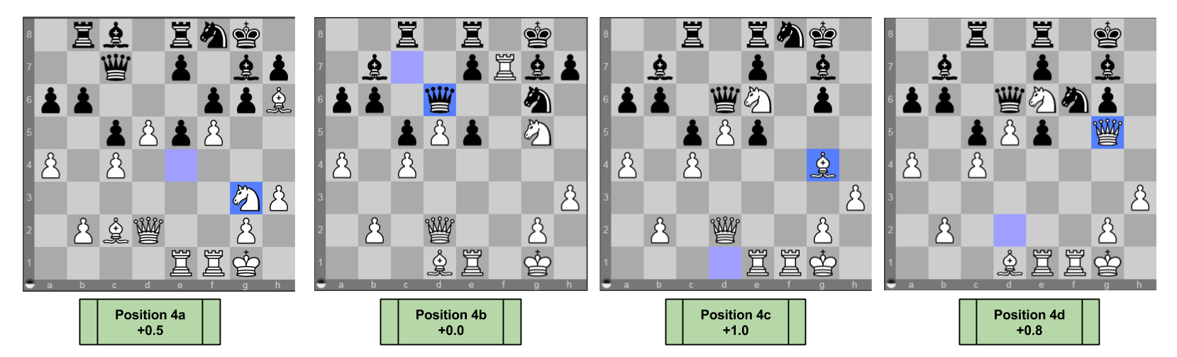
On 22 … Nf8 a plausible line may proceed: 23. Bh6 Rb8 24. Bc2 Bc8 25. Ng3 with strong positional pressure (+0.5, [pos 4a])

On 22 … fxg5 23. Nxg5 Black is faced with several defensive options, of which three stand out:

On 23 … Nf8 24. fxg6 Nxg6 25. Rf7 Black can avoid the Ne6 fork with 25 … Qd6, with a very sharp, unclear game ahead (+0.0, [pos 4b])

On 23 … Qd6 24. fxg6 hxg6 25. Ne6 White’s control of the light squares is very powerful. Play might continue 25 … Nf8 26. Bg4 (+1.0, [pos 4c])

On 23 … Nf6 24. Ne6 Qd6 25. fxg6 hxg6 26. Qg5 White’s Queen bears down on the weak g-file (+0.8, [pos 4d])

On 22 … gxf5 23. Rxf5 Black can challenge the Rook with 23 … e6 after which 24. dxe6 Rxe6. 25. Bh6 and White is comfortable (+1.0, [pos 4e])

But Black can simply capture the bishop on instead. After 23 … fxg5 24. Nxg5, Black is again faced with many defensive options.

On 24 … Rf8 Qd3 White threatens to move the rook and checkmate via Qh7. (+0.9, [pos 4f])

On 24 … Nf8 Bg4 White is poised to threaten the Rc8, and counter Black moving his e-pawn (+0.7, [pos 4g])

On 24 … e6 Nxe6 25. Qd6 Qg5 White threatens Qg7 checkmate, but this threat can be blocked (+0.5, [pos 4h])

We can again represent the above analyses graphically, as follows:

Chess Decisions Are Graph Computations

Congratulations on surviving the past two sections! We’re almost done. Take a deep breath.

The last question on our plate today is:

How should we take the above analyses and produce a move?

This seems difficult to answer. But consider the following simpler question

What is the score of our original four choices?

If we knew the score attached to our four possible moves, we would have an answer: make the move with the best possible score! 🙂

How to solve this simplified question? If we need scores in the head of the tree, graphically our task becomes propagating the already-known leaf scores back up the tree. Let’s see this in action.

We have a clear understanding of the score for the position after 22. Bh6: it is -0.2.

But what is the score after 22. Be3?

To answer this, we must first evaluate the score after 22 … gxf5. It is White’s turn, should he choose 23. Bc2 or 23. Rxf5? He should choose Rxf5, because it has a higher score! In mathematical terms, we simply take the maximum of all white moves: max(0.2, -3.0) = 0.2!

Now that we know that the state after gxf5 is +0.2, what is the score made by Be3? It is Black’s turn, should he choose gxf5 or g5? He should choose gxf5, becuase it has a lower score! In mathematical terms, we simply take the minimum of all of black’s option scores: min(0.2, 0.5) = 0.2

The above two paragraphs express the basics of the minimax algorithm. The name comes from the application of max() for White and min() for Black. Its procedure is how computers, and as I will argue brains, do chess.

Can you apply the same logic to fxg6 and Ne4? Take a moment to valuate their scores, and then come back to check your work!

Be3: 0.2
Bh6: -0.2
fxg6: 0.0
Ne4: 0.0

Now, given these scores for White’s candidate moves, which should White pick? The maximum, or 22. Be3. And that is precisely the move I chose. 🙂

Here’s a graphical representation of the above results:

It is my hope that chess decisions now remind you of lightning physics:

Takeaways

When considering possible moves, it is helpful to graph moves as nodes in a decision tree.
Analyzing chess is hard work!
When you are done constructing the decision tree, the minimax algorithm translates its data into a decision.

Appendix

If anybody is interested in how the game concluded, let me attach a link to it here for completeness. While I did win, I feel like the win was not particularly instructive. This particular moment analyzed above, however, contained a nice mix of different strategies and thereby was pedagogically useful.

1. d4 Nf6 2. c4 g6 3. Nc3 Bg7 4. e4 d6 5. Nf3 O-O 6. Be2 c5 7. d5 a6 8. a4 Nbd7 9. O-O b6 10. h3 Bb7 11. Bf4 Re8 12. Qd2 Qc7 13. Rae1 Rad8 14. Bd3 Nh5 15. Bg5 Ne5 16. Be2 Nxf3+ 17. Bxf3 Nf6 18. Bd1 Rc8 19. f4 Nd7 20. e5 dxe5 21. f5 f6 22. Be3 g5 23. b3 Rb8 24. h4 gxh4 25. Qf2 h3 26. Qg3 Kh8 27. Bh5 hxg2 28. Kxg2 Rg8 29. Bg6 Bh6 30. Rh1 Nf8 31. Rxh6 e6 32. Qh4 exf5 33. Qxf6+ Rg7 34. Kf2 Nxg6 35. Rxg6 hxg6 36. Bh6 Kg8 37. Bxg7 Qxg7 38. Qe6+ Qf7 39. Qxe5 Rf8 40. Qe6 Qxe6 41. Rxe6 Kg7 42. Rxb6 Rf7 43. b4 cxb4 44. Rxb4 Kf6 45. Rb6+ Kg5 46. c5 f4 47. Ne4+ Kh4 48. Nd6 Bxd5 49. Nxf7 Bxf7 50. c6 Be6 51. c7 Bf5 52. Rxg6 Kh5 53. Rg8 1-0

Average Causal Effect

January 21, 2015March 21, 2017kevinbinz 1 Comment

Followup To: Potential Outcome Models
Part Of: Causal Inference sequence
Content Summary: 900 words, 9 min read

Recap

Our takeaways from last time:

Questions of causality have interesting links to “what if” questions (counterfactuals)
We can construct a Possible Outcomes model that deploys counterfactual reasoning to explain observed effects
If we reverse the direction of a Possible Outcomes model, we see that observed reality only partially determines our counterfactual knowledge.
If we look carefully at the relationship between observed variables and their counterfactual implications, we can begin to see a pattern.

Today, we will connect our Possible Outcomes Model back to causality. But first, we must address questions of scale!

Scaling Up Potential Outcome Models

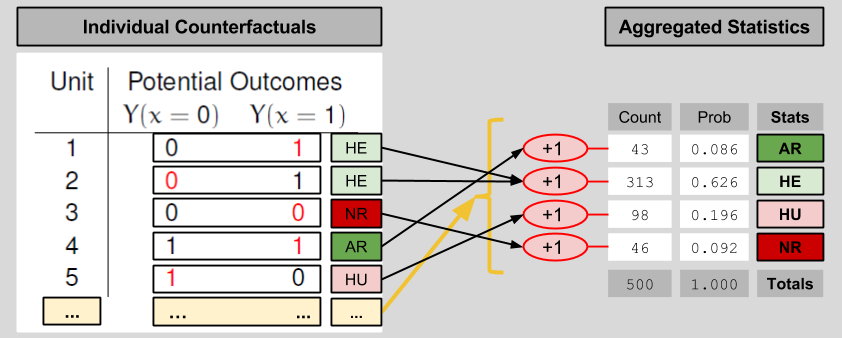
In order to get a sense for the performance of the drug as a whole, one needs to view its effects on a larger population. The above table has N=5 subjects. Let’s imagine 500 subjects instead. Fortunately, if we don’t want to deal with 500 row tables, we can aggregate the data into a shorter entry. Here’s one possible way to compress a large counterfactuals table into four entries:

We compress the observables table in an analogous manner:

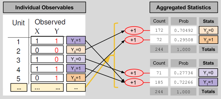
These statistical results relate to each other in the following way:

Average Causal Effect

Let us now shift our gaze from machinery to our original motivation. How might we use potential outcome models to estimate causal effect? If most of our patients are of type NR or AR (Never/Almost Recover), that would suggest that our drug is exerting negligible causal muscle over the patients. However, a drug that indexes many patients of type HE (Helped) seems to have an effect. Conversely, a drug that creates many HU (Hurt) patients can also be said to have a medical impact. Let us create one measure to index both; let Individual Causal Effect (ICE) represent:

ICE = Y₁ – Y₀

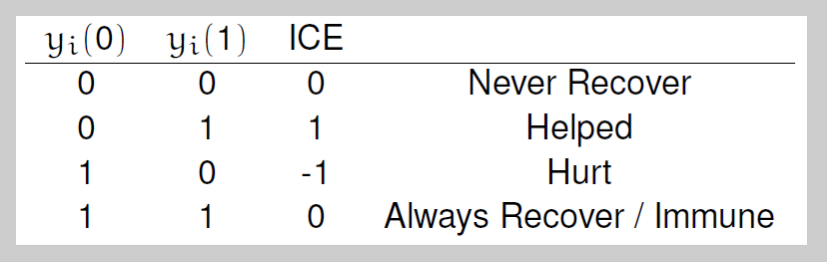
Another way of putting the above paragraph, then, is that causally-interesting patients are those with a non-zero ICE score.

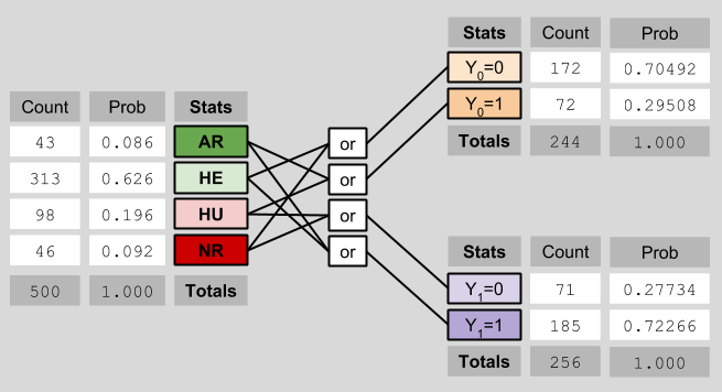
As we scale up our model, our causal measure must follow suit. Let Average Causal Effect (ACE) represent:

ACE = P(HE) – P(HU)

In our case (see the diagram about ICE), the ACE = 0.626 – 0.196 = 0.43.

Learning ACE Bounds

Let’s put on our Learning Mode Glasses, and recall that we are unable to observe P(HE) nor P(HU). Instead, we can only view X and Y. What can we learn about the ACE in this context? It is tempting to say “nothing”, since we cannot uniquely determine the counts of the four outcome types. But this would be a mistake, for we can in fact establish bounds for our ACE.

The lower bound of the ACE occurs when the maximum possible number of observed outcomes are ascribed to Hurt people, and the minimum possible number of observed outcomes are ascribed to Helped people:

Thus, the lowest possible value of the ACE is 0.000 – 0.286 = -0.286.

Analogously, the upper bound of the ACE is determinable by imagining a scenario with as few Hurt people, and as many Helped people, as possible:

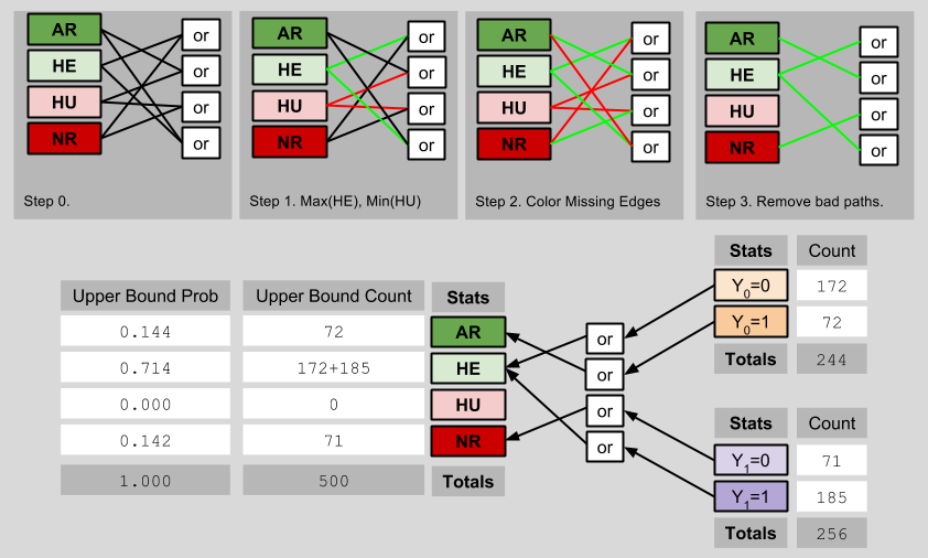
The highest possible value of the ACE is therefore 0.714 – 0.000 = 0.714. Thus, we can see that (despite not knowing the true ACE), we have shrunk its possible values from [-1, 1] to [-0.286, 0.714]. Importantly, this smaller fence still contains the true ACE of 0.43.

Transcending ACE Bounds

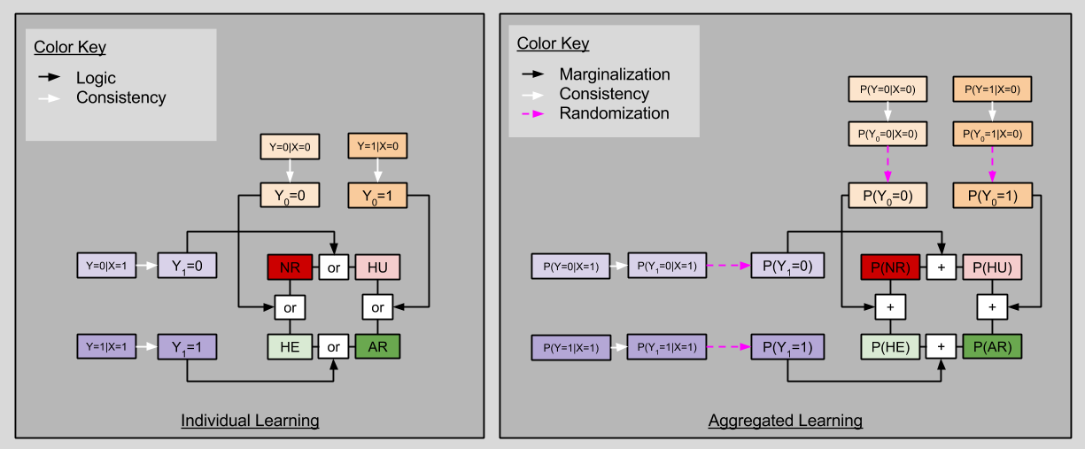
Can we do better than this? Yes. Let us recall an axiom we used to build our Potential Outcomes Framework:

Consistency Principle: Y = Y₁* X + Y₀*(1-X)

This principle is saying nothing more than that the red numbers on our potential models diagrams must match:

It turns out that, if you are willing to purchase an assumptions, you can estimate the true ACE from observed data alone.

Randomization Assumption: selection variable X is independent of the counterfactual table (X ⊥ Y₀, Y₁)

If the Randomization Assumption is true, then we may derive the following startling fact:

P(Y=i|X=1)

= P(Y₁=i|X=1) # Because of Consistency Principle

= P(Y₁=i) # Because of Randomization (X ⊥ Y₁)

= P(Y₁=i, Y₀=1) + P(Y₁=i, Y₀=0) # Marginalization over Y₀

When i=0, we have P(Y₁=0) = P(HU)+ P(NR). When i=1, we have P(Y₁=1) = P(HU)+ P(NR)

By the same logic, we can condition on X=0:

P(Y=i|X=0)

= P(Y₀=i|X=0) # Because of Consistency Principle

= P(Y₀=i) # Because of Randomization (X ⊥ Y₀)

= P(Y₀=i, Y₁=1) + P(Y₀=i, Y₁=0) # Marginalization over Y₁

When i=0, we have P(Y₀=0) = P(HE)+ P(NR). When i=1, we have P(Y₀=1) = P(AR)+ P(HU)

These four facts together exhibit startling similarities to one of our results from last time:

Notice that, although we can never uniquely determine say P(HU) from observables alone, we can estimate the ACE directly!

P(ACE)

= P(HE) – P(HU)

= P(HE) + P(AR) – [P(HU) + P(AR)]

= P(Y₁=1) – P(Y₀=1)

Let’s see this in action. Recall our original data, reproduced in aggregated form below:

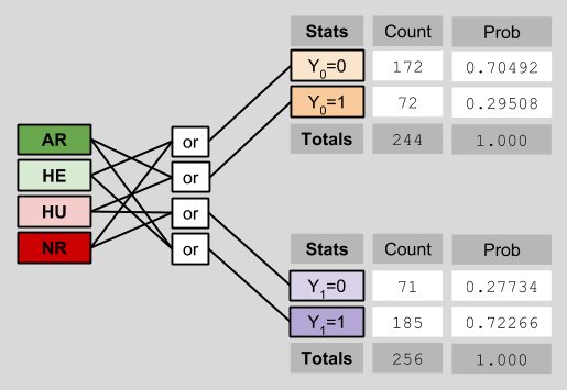
Notice that I have explicitly removed the counterfactual data previously visible on the left side of the diagram. This deletion reflects the fact that counterfactual data is intrinsically opaque to us. This depressing fact is known as the Fundamental Problem Of Causal Inference.

Here, we can estimate the ACE as follows:

P(Y₁=1) – P(Y₀=1)

= 0.72266 – 0.29508

= 0.427528

If that’s not close to the ACE true value of 0.43, I don’t know what is. 🙂

Takeaways

Data aggregation statistics are a useful way of summarizing large counterfactual/observable tables.
Rubin’s potential outcome model informs philosophical questions of causality through his Average Causal Effect (ACE) measure
In real-world scenarios, where counterfactual data is opaque to us, we can still derive upper and lower bounds for the ACE
If we are willing to assert the independence of sampling processes, however, we are able to estimate the ACE directly!

Fewer Lacunae

Distilled, Integrative Research

Author kevinbinz

[Sequence] Game Theory

Computational Trinitarianism

Nash Equilibria

An Introduction To Prisoner’s Dilemma

Getting Real With Continued Fractions

Bridging the Is-Ought Gap

The Psychology Of Chess

The Chess SuperTree

Decision Trees In Chess

Average Causal Effect