Getting Real With Continued Fractions

April 29, 2015March 23, 2017kevinbinz Leave a comment

Content Summary: 600 words, 6 min read

And now, an unprovoked foray into number theory!

Simple Continued Fractions (SCFs)

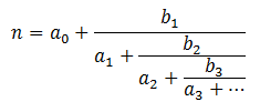
Have you run into simple continued fractions in your mathematical adventures? They look like this:

Let $A$ represent the coefficients $(a_0, a_1, a_2, a_3, ...)$ and $B = ( b_1, b_2, b_3, ...)$ . If you fix $B = (1, 1, 1, ...)$ you can uniquely represent $n$ with $A(n)$ . For example:

$n = \frac{415}{93} = 4+\frac{1}{2+\frac{1}{6+\frac{1}{7}}}$

$A(n) = (4,2,6,7)$

Let us call $A(n)$ the leading coefficients of n. Here we have represented the rational $\frac{415}{93}$ with four coefficients. It turns out that every rational number can be expressed with a finite number of leading coefficients.

Continued Fractions- Number Properties v1

Irrational Numbers

Life gets interesting when you look at the leading coefficients of irrational numbers. Consider the following:

$A(\phi) = (1, 1, 1, 1, 1, 1, 1, ...)$

$A(\sqrt{19}) = (4, 2, 1, 3, 1, 2, 8, 2, 1, 3, 1, 2, 8, ...)$

$A(e) = (2, 1, 2, 1, 1, 4, 1, 1, 6, 1, 1, 8, ...)$

$A(\pi) = (3, 7, 15, 1, 292, 1, 1, 1, 2, 1, 3, 1, ...)$

First note that these irrational numbers have an infinite number of leading coefficients.

What do you notice about $A(\phi)$ ? It repeats, of course! What is the repeating sequence for $A(\sqrt{19})$ ? The sequence $213128$ .

How about $A(e)$ ? Well, after the first two digits, we notice an interesting pattern $211$ then $411$ then $811$ . The value of this triplet is non-periodic, but easy enough to compute. The situation looks even more bleak when you consider the $A(\pi)$ …

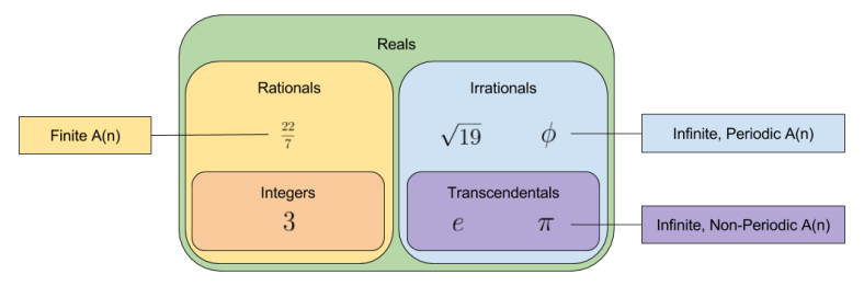
Thus $\phi$ (golden ratio) and $\sqrt{19}$ feature repeating coefficients, but $\pi$ and $e$ (Euler’s number) do not. What differentiates these groups?

Of these numbers, only the transcendental numbers fail to exhibit a period. Can this pattern be generalized? Probably. 🙂 There exists an unproved conjecture in number theory, that all infinite, non-periodic leading coefficients with bounded terms are transcendental.

Continued Fractions- Number Properties

Real Approximation As Coefficient Trimming

Stare the digits of $\pi$ . Can you come up with a fraction that approximates it?

Perhaps you have picked up the trick that $\frac{22}{7}$ is surprisingly close:

$\pi = 3.14159265359$

$\dfrac{22}{7} = \textbf{3.14}285714286$

But could you come up with $\frac{22}{7}$ from first principles? More to the point, could you construct a fraction that comes yet closer to $\pi$ ‘s position on the number line?

Decomposing these numbers into continued fractions should betray the answer:

$A(\pi) = (3, 7, 15, 1, 292, 1, 1, 1, 2, 1, 3, 1, ...)$

$A\left(\dfrac{22}{7}\right) = (3, 7)$

We can approximate any irrational number by truncating $A(\pi)$ . Want a more accurate approximation of $\pi$ ? Keep more digits:

$(3, 7, 15, 1) = A(\dfrac{355}{113})$

$\dfrac{355}{113} = \textbf{3.141592}92035$

I’ll note in passing that this style of approximation resembles how algorithms approximate the frequency of signals by discarding smaller eigenvalues.

About π

Much ink has been spilled on the number $\pi$ . For example, does it contain roughly equal frequencies of 3s and 7s? When you generalize this question to any base (not just base 10), the question becomes whether $\pi$ is a normal number. Most mathematicians suspect the answer is Yes, but this remains pure conjecture to-date.

Let’s return to the digits of $A( \pi )$ . Here is a graph of the first two hundred:

Do you see a pattern? I don’t.

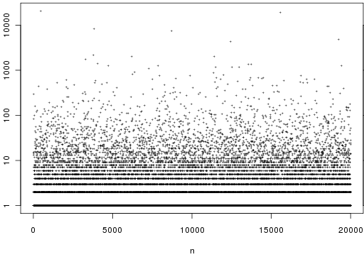
Let’s zoom out. This encyclopedia displays the first 20,000 coefficients of $A( \pi )$ :

So $A(\pi)$ affords no obvious pattern. Is there another way to generate the digits of $\pi$ such that a pattern emerges?

Let quadratic continued fraction represent a number $n$ expressed as:

Set $A = (1, 2, 2, 2, 2, ... )$ . Here only $B = ( b_1, b_2, b_3, ...)$ is allowed to vary. Astonishingly, the following fact is true:

$B\left(\dfrac{4}{\pi}\right) = (1, 3, 5, 7, 9, 11, 13, 15, 17... )$

Thus, continued fractions allow us to make sense out of important transcendental numbers like $\pi$ .

I’ll close with a quote:

Continued fractions are, in some ways, more “mathematically natural” representations of a real number than other representations such as decimal representations.

Bridging the Is-Ought Gap

April 2, 2015April 7, 2017kevinbinz Leave a comment

Part Of: Demystifying Ethics sequence
Prerequisite: An Introduction to Propriety Frames
Content Summary: 1400 words, 14 min read

Introduction

This article presents a theory of normatives. It is not a complete theory (it does not even describe implementation), nor does it answer a number of important objections. I sketch it, in its current state, in order to motivate the claim that explaining normatives is possible.

Hyperpoints

Consider again the problem of describing locations in a space. In a two dimensional space, any coordinate system I use (e.g., Cartesian or polar) require two pieces of data to uniquely specify the location. In a space with three degrees of freedom, three points of data are required. Call this symmetry between dimensionality and data the data-dimension bridge.

Your brain is embedded in a three dimensional space, and your visual system evolved in this context. It is just as mathematically meaningful to discuss locations in a 17D space, despite the fact that you lack the mental equipment to visualize it.

Take this argument to an extreme. The universe contains approximately 10^82 atoms. If we suppose there are 100 interesting facts we can name for every atom, this means that we need 10^84 data points to describe the universe. Given our data-dimension bridge, this means that the entire universe can be described by the location of one point in a (10^84)D space.

Such hyperpoints turn out to be a surprisingly versatile concept, appealed to frequently by mathematicians. They were first introduced in an inaugural lecture by Bernhard Riemann in 1854.

Propriety Frames

Main Article: An Introduction To Propriety Frames

Our everyday lives are immersed in highly structured interactions. Much of these community expectations are taken for granted; they are practically invisible to us. But if you travel to a culture sufficiently remote from your own, or spend much time around people suffering from Asperger’s syndrome, and you can begin to build an appreciation for these culturally-approved roles.

Consider a typical evening spent at a fancy restaurant. If I asked you to come up with a complete list of examples of things that would surprise you, how long do you think that list would be? Consider some representative examples.

The waiter states he is not in the mood to take your order.
Several guests are engaged in a foodfight.
An expensive item on the menu is marked as free of charge.
Instead of payment, the manager comes out to request that you wait tables next weekend.
The food is dumped directly on the table.
On taking a bite, you realize that your meal is actually plastic: an artistic creation designed purely for visual effect.

The length of the list corresponds to the volume of knowledge embedded within your brain’s social intuitions.

Social psychology likes to speak of frames as a useful way to bundle collections of facts together. We can say that our restaurant experience is defined as the intersection of three different frames: host-guest, place of business, eating. Each of the above surprises are produced by a violation of one of these frames.

Propriety Frames- Restaurant Example (3)

When a mother instructs her son to not yell in the store, the child installs an update to his Shopping frame. When a family exchanges gossip around a campfire, they are doing so in part to synchronize their propriety frames.

Mental Hyperpoints

Time to synthesize the above. Each social frame can be decomposed into a collection of facts. Thus, a person’s social intelligence can be fully described by a hyperpoint in frame-space.

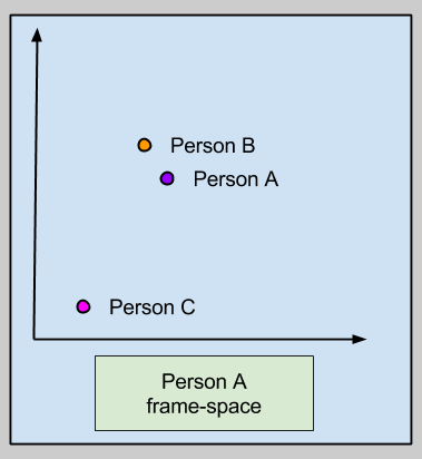
In fact, we can represent any mental process in terms of hyperpoints. In the following graphic, we are representing the social memory, semantic memory, and perceptual memory.

Take a moment to appreciate this graphic. Every sentence you utter, every subtlety of your body language, every friendship you have ever formed: the totality of your life as an organism is captured as a single point in behavior-space.

Did you notice how Person A only encodes other people in behavior-space? This is because human beings do not have direct access to one another’s mental lives. That said, we can imagine that knowledge of another person’s behavior may let us estimate the social rules they hold as legitimate.

A Theory Of Normatives

Let’s switch gears. What does it mean for somebody to say “you should buy this stock” or “you should not blackmail your coworkers”?

We call statements with “should” in them normative language. These contrast with descriptive statements of reality. David Hume noticed this distinction clearly, and formulated what is now known as the is-ought gap:

In every system of morality, which I have hitherto met with, I have always remarked, that the author proceeds for some time in the ordinary ways of reasoning, and establishes the being of a God, or makes observations concerning human affairs; when all of a sudden I am surprised to find, that instead of the usual copulations of propositions, is, and is not, I meet with no proposition that is not connected with an ought, or an ought not. This change is imperceptible; but is however, of the last consequence. For as this ought, or ought not, expresses some new relation or affirmation, ’tis necessary that it should be observed and explained; and at the same time that a reason should be given, for what seems altogether inconceivable, how this new relation can be a deduction from others, which are entirely different from it.

With this backdrop, I would like to propose the following three-part theory of normatives.

First, normatives are nothing more than hyperpoints in frame-space, tagged by a separate module with a “should” label. Call these marked hyperpoints normative attractors. As evidence, consider that every statement of “ought” can be cast back into descriptive language (“you should do X” can be translated into “good people do X”).

Second, normative attractors are fed into our motivational subsystems. The word “ought” is not just a fun word to throw around, it evolved to promote behavioral change.

Third, normatives co-evolved with natural language. Recall the functional purpose of language: to allow humans to exchange mental information. Mental information about the world (human semantic memory) required no additional hardware to synchronize: perceptual psychophysics provides a sufficient reference point. But coordinating social frames had no such advantage, and required new hardware (the attractor).

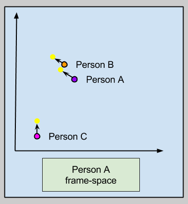
Let us call this toy hypothesis the Frame Attractor theory of normatives. Here’s an illustration; where the yellow attractor represents Person A’s vision of optimal behavior (e.g., Buddha, Jesus, “being nice”, etc):

Disaggregated Attractors

It is a virtue of explanatory models to consume prior considerations under a more comprehensive framework. I have used this model to improve my understanding of why conflicts happen, and how to resolve them peaceably. This is left as an exercise to the reader. 🙂

In the above image, consider the plight of Person C. Is the sheer distance between their behavior and the norm motivating?

In Normative Therapy, I state the following:

Let me zoom in on one “population subset”: the sociopath. Such an individual is biologically incapable of meeting aggregate-level normative impositions such as “everyone should care about the well-being of those around them”. The argument here, is that normative impositions should be explicitly tailored to the individual situation; for people like sociopaths, this would be something like, “sociopath X should put herself in situations where her non-empathic behavior can be held accountable”.

This observation, and the argument underlying that post, suggests that it may be advisable to disaggregate normatives. If the goal of morality to more effectively move people towards the normative attractor, perhaps innovation in cultural technology will permit stable individuated attractors, like this:

The above example uses disaggregated normatives as lures to attract people towards The Goal. But this is not the only use of such a mechanism. Perhaps we could also train personal-attractors in a more diverse ethical setting with multiple Goals. But, for now, let me leave such a question for another day.

Takeaways

Thinking about complex ideas as locations in a high-dimensional space (hyperpoints) is a surprisingly powerful conceptual tool.
Complex community rules are most likely implemented via a particular memory system that encodes social frames.
The Frame Attractor theory of normatives is grounded in three principles
1. “Ought language” are hyperpoints in frame-space, tagged with a “should” label. Call these normative attractors.
2. Normative attractors are fed into our motivational subsystems.
3. Normatives co-evolved with natural language.
This theory can be used to explain other arguments, such as my argument in support of person-specific normatives.

The Psychology Of Chess

March 29, 2015June 27, 2017kevinbinz 1 Comment

Part Of: Chess sequence
Followup To: The Chess SuperTree
Content Summary: 1400 words, 14 min read

Dual Process Cognition: Working Memory

Chess engines operate by generating a decision tree, pruning irrelevant branches, assigning scores to the leaves, and consulting the minimax oracle for an optimal decision.

But when we switch from silicon to grey matter, we notice that the human mind is structured differently. We can be meaningfully divided into two selves: a fast, autonomic, associative mind and a slow, serial, conscious mind. What’s worse, the content of our “more rational” self is small – System II is grounded in working memory, which can hold 7 +/- 2 chunks of information.

Working memory span is highly correlated with IQ. Keith Stanovich, in his Rationality and the Reflective Mind, claims that intelligence can be understood as a cognitive decoupling; that is, highly intelligent people are able to evaluate more hypothetical scenarios faster, and keep those explorations firewalled from one’s modeling of the current reality.

While playing chess, the ability to construct a decision tree is a conscious, effortful task. In other words, decision trees are instantiated within your System II working memory during game play.

Dual Process Cognition: Somatic Markers

If decision trees are consciously maintained, what is the basis of score evaluation functions? Recall that machine learning accomplishes this by virtue of training feature vectors and weight vectors. Suppose these vectors can contain two millions numbers each. Every time the engine is asked to evaluate a position, it will compute a dot product: scan over the vectors, and for each value record its product.

With decision trees, I can remember keeping various alternatives in my head. Not so with producing decision scores. Nothing in my gameplay experience feels like I am computing two million numbers with every move. This suggests that score evaluation functions happen within the subconscious, massively parallel System I.

But what does evaluating a position feel like? Two phenomenological observations are in order:

Playing chess is a highly intuitive, emotional affair. Positions in which we have a strong advantage feel good, moves that lead us into checkmate feel scary, and the objectively optimal move tends to produce the most positive feeling. In other words, emotion is the mediator of chess skill. This is an expression of the somatic marker hypothesis.
Explaining chess moves tends to naturally flow in a non-mathematical language, where reasons are considered the final authority over decision making. I am better able to remember “White is better because he has an attack” instead of “White is 20% more likely to win the game”.

We’ll return to these suggestive observations in a little bit.

Is Scoring Cardinal Or Ordinal?

In economic theory, all decisions are mediated by a psychological entity called utility. (I introduce this concept in this post). Neuroeconomics is an attempted integration between economics, psychology, and neuroscience; it tries to get at how the brain produces decisions. Within this field, there is a live debate whether the brain represents utility cardinally (e.g., 3.2982) or ordinally (e.g., A > B and B > C).

Consider again how chess engines compute on the decision tree. The minimax algorithm pushes leaf nodes up the tree, merging results via the min() or max() operation. Whereas engines perform these operation against cardinal score nodes (e.g., in fractions of a pawn called centipawns), this need not be the case. Taking the max(A, B) does not require knowing the precise value of A and B. It is sufficient to know that A > B. In other words, minimax can also work against an ordinal scoring scheme.

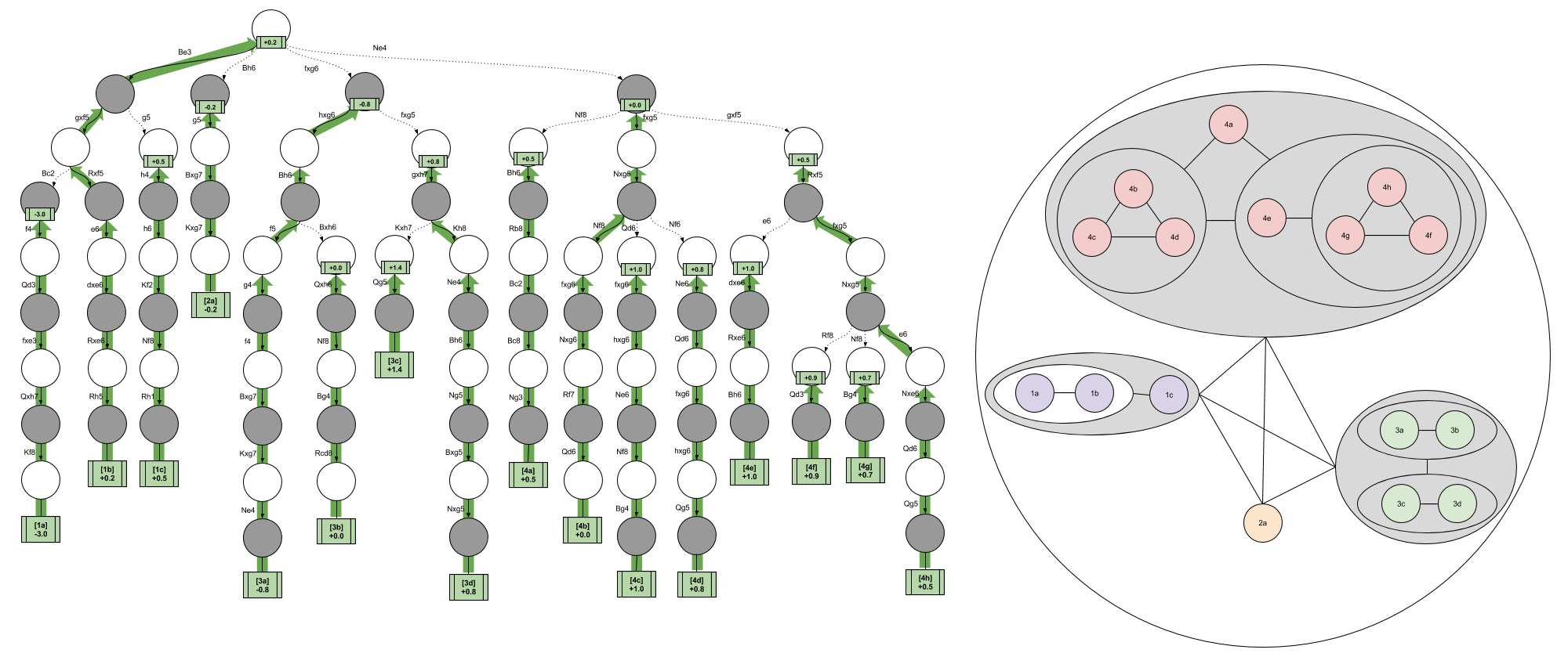
The implications of an ordinal scoring scheme becomes more apparent if you view the minimax algorithm from a comparison perspective. In the following image, white spheres represent White decisions (maximization) and gray spheres represent Black decisions (minimization).

It is possible to think of image on the left as a “side view” of the minimax algorithm. With this geometric interpretation, the right image becomes a “bottom view” of the exact same algorithm. Pause a moment here until you convince yourself of this.

Consider the nested spheres containing the purple nodes. These represent three leftmost threads in the decision tree: { { 1a vs 1b } vs 1c }. Do we need to know the value of { 1a vs 1c } or { 1b vs 1c }? If we knew both facts, we could surely have enough information to implement minimax. But this “easy solution” would require a total ordering, which is prohibitively expensive. We instead need to resolve the { 1a vs 1b } fact, after which we can compare the result to 1c.

So the brain could choose to evaluate positions ordinally or cardinally. Which technology does it employ in practice?

I don’t know, but I can recommend a test to divine the correct answer. The order in which cardinal scores are generated is unconstrained: a chess player with a cardinal function can evaluate any position at any time. In contrast, the order in which ordinal scores are generated is highly constrained (if we assume a non-total ordering). A brain that implement ordinal evaluations cannot physically evaluate the 1c thread until it has evaluated { 1a vs 1b }. Thus, if we were to study the speech and subjective experiences of a multitude of chess players, we could hope to learn whether their creative abilities are constrained in this way.

The State Comparator & Distinguishing Features

Consider again the feature-weight dot product model of score functions. If I were to evaluate two very similar functions, the dot product would necessarily be very similar: only a few dozen features may meaningfully diverge in their contribution to the final output. Call these uniquely divergent features the distinguishing features.

A computer engine will compute similar dot products in their entirety (with the exception of position that are exactly the same, see transposition tables); it strikes me as very likely that the brain (a metabolic conservative) typically only retains a representation of the distinguishing features. In other words, the “reason-based natural language” that humans produce when we evaluating gamelines draws from a cognitive mechanism that recognizes that features close in distance to the KingSafety category tend to be the relevant ones.

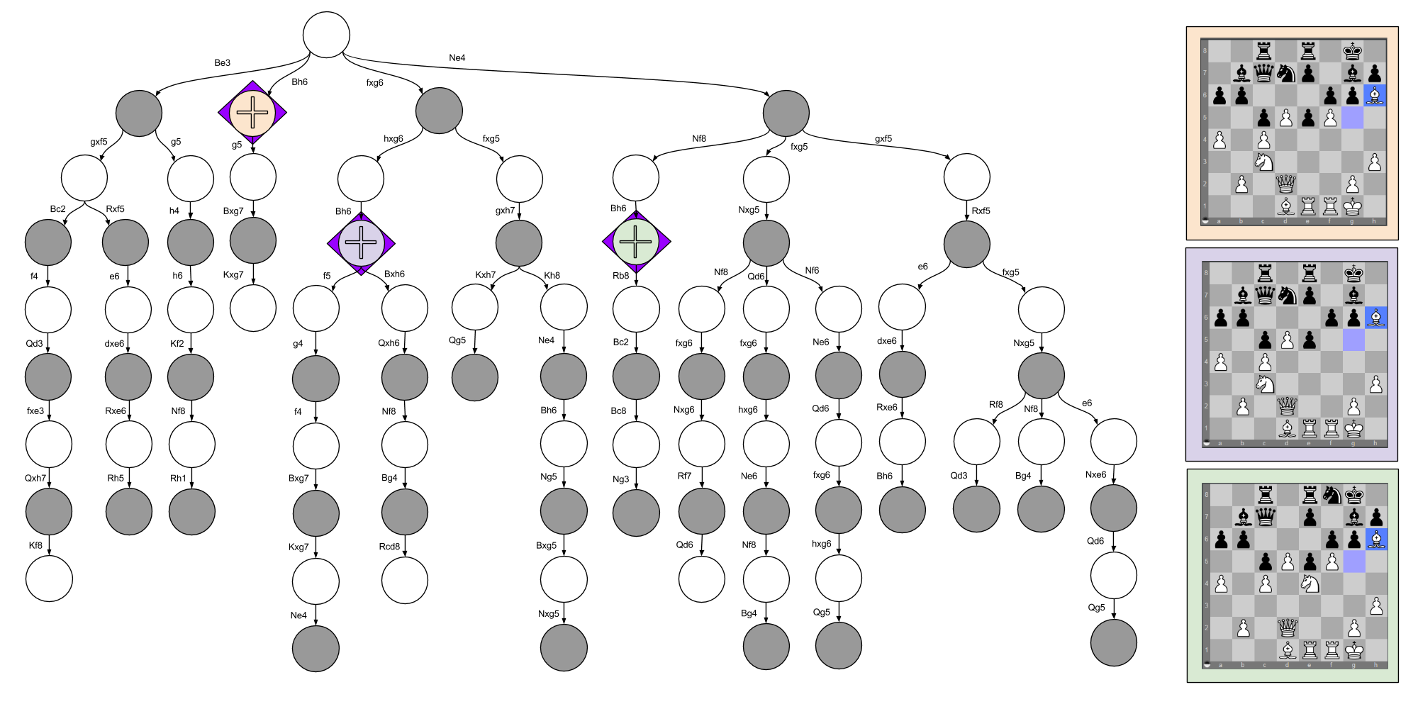
In the discussion of Decision Trees In Chess, I discuss four different moves. The insightful reader may have noticed that I moved my Bishop to the h6 square in three separate situations. These considerations happen at three locations in the decision tree:

While a chess engine may score each position repetitively, each score computation will be very similar. Only two features really stand out:

The purple node is different from the orange node because the former has traded off two pawns.
The green node is different from the orange node because the former has made two Knight moves to attack & defend the Kingside.

If you consult the minimax graphic above, you’ll see that my preference ordering is { Green > Orange > Purple }. I would explain this in language by appealing to the relevant differences (e.g., “the pawn trade frees his pawns to control the center”). To me, this is evidence for a state comparison tool that is able to zoom in on distinguishing features.

The Move Generator & Representative Lines

Another distinction between human and computer decisions in chess seems to lie in how the decision tree is approached. Engines like Stockfish typically have a getLegalMoves() function that fleshes out the entire branching structure, and then (extremely) sophisticated pruning techniques are used to make truly deep evaluations possible of the interesting lines. It is possible that nonconscious Type I processes in humans do something comparable, but this strikes me as unlikely. Rather than an eliminative approach to the SuperTree, it seems to me that humans construct representations gradually.

Specifically, I suspect that humans have a Type I statistical mechanism that generates a few plausible moves for a given position. Consider the following subset of a decision tree I examined previously:

Each orange rectangle represents moments when I simply stopped considering alternatives; these representative lines are depth-oriented in nature. I suspect the ubiquity of these representative lines can be explained by appealing to serial application of the MoveGenerator, and the sheer difficulty humans have in maintaining a complex tree in working memory.

Takeaways

The brain represents decision trees largely in working memory (a conscious System II process)
Massively parallel System I processes are how the brain computes position scores, which are encoded in emotion.
While computers represent scores as numbers, it is possible the brain represents scores as preferences (an ordinal system).
The brain, being allergic to duplicate computations, contains a State Comparator which isolates distinguishing features within similar positions.
Rather than pruning a complete decision tree like computers, the brain an intuitive, System I, Move Generator to construct a plausible sub-tree.

The Chess SuperTree

February 28, 2015June 27, 2017kevinbinz Leave a comment

Part Of: Chess sequence
Followup To: Decision Trees In Chess
Content Summary: 1500 words, 15 min read

Chess Is A Nested Algorithm

In An Introduction To Chess, I introduced you to the basics of chess analysis: how to tell when one position is better than another. Specifically, we looked at material, pawn structure, space, king safety, piece development, piece cohesion, and initiative. These ways of thinking about different chess positions were combined into a score. The first aspect of chess thought lies in the maturation of such an scoring function.

In Decision Trees In Chess, I introduced you to the basics of chess decision making: how to evaluate different alternatives when you are not sure what to do. Specifically, we looked at how imagining different scenarios can be represented in decision trees, how these trees ultimately use scoring functions in their leaf nodes. These decision trees produce decisions after application of the minimax algorithm.

Together, scoring functions and decision trees describe the entirety of what it is to do chess. Had this series been written by world champion Magnus Carlsen, I submit that even he could communicate effectively using this two-part framework. The only things that need be different would be his analysis (his scoring function would be more accurate) and his choice of alternatives to analyze (his considered choices would contain fewer bad alternatives). In other words, skill in chess is not doing more than score functions and decision trees. It is doing them well.

Two Kinds Of Score

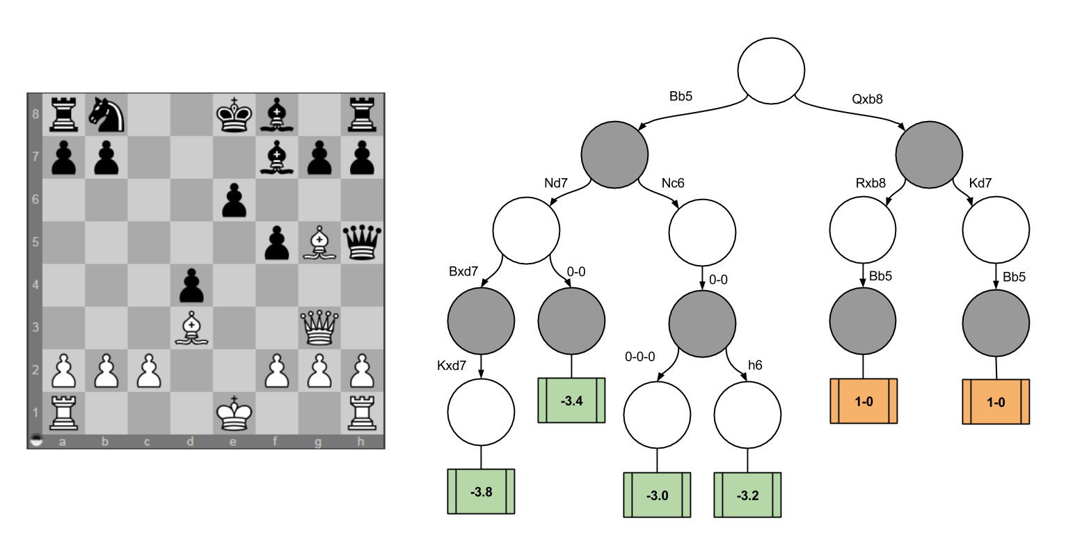
Consider the following. White’s turn, can you find mate in two moves?

The solution to this puzzle, displayed on the rightmost decision tree, is Qxb8+. If Black recaptures, White checkmates with Bb5# (note that the Bg5 prevents Black’s king from escaping (and if Black runs away Kd7, he is met with the same fate).

Now, imagine if White had not found this clever solution immediately. Suppose White instead tries to attack Black with Bb5+. White’s reflections could lead him to consider the other decision tree, which ultimately values Bb5 as -3.2 points (do you see why the minimax algorithm requires this to be the case?)

Consider the returned values (1-0 WIN) for Qxb8+, and (-3.2) for Bb5. This incongruity is itchy. Why would the scoring function return different types of answers depending on the position?

Meet The SuperTree

Imagine for a moment the decision tree for all chess games. Call this object the SuperTree. What does it look like?

Consider the following facts:

On move zero, all chess games ever begin in the same position.
After white’s first move, all chess games ever are in one of twenty possible positions (White has 20 legal moves)
After Black’s first move, all chess games ever are in one of four hundred possible positions (20*20)
All chess games ever conclude with a result (White wins, Black wins, or tie). Some games finish quickly, others take many moves.

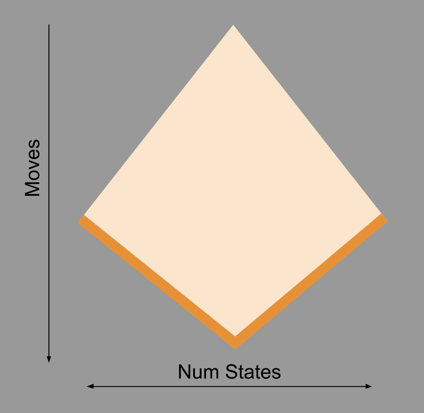
These facts can be consolidated into the following visualization:

Consider the top of the SuperTree: as we move our gaze downwards, its width increases. This corresponds to our observation above that, as more moves are made, the number of possible positions rapidly increases.

Why then does the number of possible positions decrease as we move into the endgame? Well, you have surely noticed how endgames tend to feature fewer pieces. Consider all chess games that have transitioned into King+Queen vs. King. There are only a few thousand ways to place these three pieces on the board (64*63*62 = 249,984 is an upper bound). Fewer pieces means fewer states (which is why the Supertree is shown as a diamond, not of a triangle).

At the end of every game, at the end of a game tree, are result nodes. This are represented by the dark orange boundary.

We have so far analyzed two game positions: my game from the Decision Trees In Chess post, and the Mate-In-Two position above. Since the above cartoon claims to comprise all chess games that can ever be played, let’s see how these games fit into the SuperTree.

On the left, we see that the Mate-In-Two game line from this post is shorter: this reflects that it (presumably) terminated in the early middlegame, whereas my opponent in the last post survived until the 53rd move.

On the right, we see the decision trees we constructed at moments in each of these games. Pay attention to the coloring of these trees: in the earlier analysis, our endpoints we numerical scores (green) which propagate up to the top of the triangle. In today’s analysis, our endpoints contain a mixture of numerical scores (green) and final results (orange). In this case, by minimax logic, the orange style of result successfully propagated to the top of the decision tree.

Can Chess Be Solved?

Final results, like numerical scores, propagate up a decision tree. If we start at the end of chess games, and work our way backwords, could we color the entire cartoon orange? Could we banish these numerical scores and solve chess? By “solve chess”, I mean be able to prove perfect play; that is, to be able to prove, from any position, the correct move (including move 1).

Lest I be accused of dreaming of something too implausible, precisely this has been done for games like Checkers and Connect-4 (more examples here).

It turns out that chess has been partially solved: computer scientists have managed to solve all games that land in King+Queen vs. King positions. Don’t believe me? Go here, and experience for yourself what it is like to play against God.

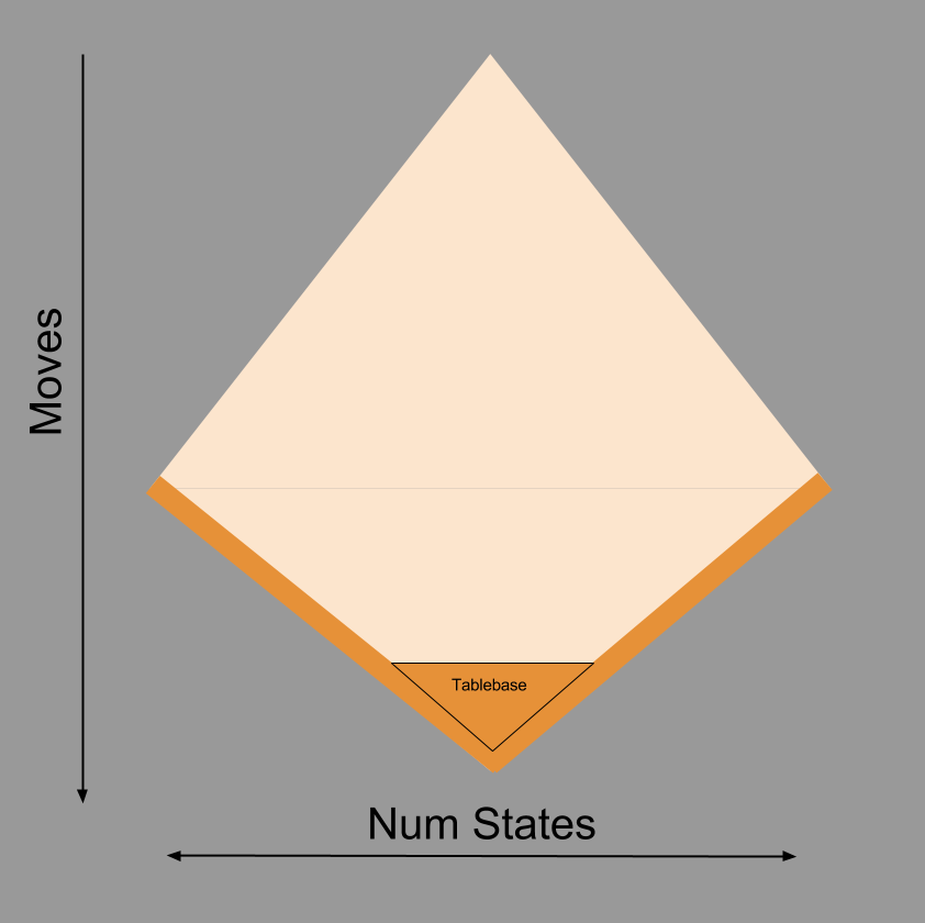
We can visualize on our cartoon how computer scientists have managed to “pull orange upwards” in an attempt to solve the SuperTree. These results are typically referred to as tablebases.

Why haven’t tablebases reached the top of the SuperTree? Compare the size of tablebases as we increase the number of pieces. A three-piece tablebase would include, for example, our classic example of King+Queen vs. King. Such a tablebase only requires 62 kilobytes of memory. But consider what happens when we accomodate more pieces:

Number Of Pieces	Tablebase Size (Bytes)
3	62,000	62 kB
4	30,000,000	30 MB
5	7,100,000,000	7.1 GB
6	1,200,000,000,000	1.2 TB
7	140,000,000,000,000	140 TB

To my knowledge, to date our modern supercomputers have failed to construct a complete 8-piece tablebase. Chess begins with 32 pieces. From the table above, when do you think the human race will possess enough computing resources to implement a 32-piece tablebase? 🙂

A Role For Numeric Scores

We now see why our scoring function cannot return game results for most moves in our path.

Consider the case where the results of the Supertree propagate upwards in a completely unpredictable manner. In this situation, we could do no better than rolling a dice to make our move, because no move can increase or chances of winning (or losing, or drawing).

But chess is not like this. Suppose you convince two evenly-matched players to play 100 games, and you remove the queen from the first player’s starting position before each match begins. The second player will probably win many more than 50 games. This tells us that chess results are not completely unpredictable. Locations in the SuperTree in which one player has a material advantage have an above-average chance of leading to a Win result, just as material disadvantages tend to balance the scale towards the Lose result. Given this window of improved predictability, we can prefer moves that improve our material situation.

Most moves in chess, regrettably, do not yield a material advantage. Can we do better than rolling the dice? Do there exist materially-equal positions where, when given to evenly-matched players, one player will win more frequently? Of course there are. We met some of these measures in An Introduction To Chess, for example:

Pawn structure. Some pawn configurations are more stable and defensible than others.
Space. Some pawn configurations allow a player relatively more room to maneuver.
King safety. How many defensive resources does a player have near his King?
Piece development. At what rate has one managed to bring pieces into the fight?
Piece cohesion. Are one’s pieces working together well?
Initiative. Who is making more threats, and dictating the course of the game?

Skill in chess is nothing more, and nothing less, than this: the ability to discover new features (patterns in the Supertree) and the ability to “mix & match” all features to produce a single move recommendation.

This is why our “green” numeric results are are so vital. Despite not knowing the true state of the underlying SuperTree, iteratively maturing your score function provides a player with an increasingly confident prediction of the SuperTree’s true value. In other words, these aggregations of different features comprise a heuristic flashlight that gives clues about the SuperTree.

Takeaways

Chess decisions are made via a nested algorithm.
- At the higher level, a player must compute a decision tree, and make decisions by rolling up the leaf scores via the minimax procedure.
- At the lower level, for each node in the decision tree, a player must invoke a scoring function to evaluate the desirability of that position.
Some decision trees can be evaluated as Win/Lose/Draw, rather than a particular number.
The SuperTree – the decision tree that contains all possible moves of any possible game – is a useful way to think about the game of chess.
We can think of specific games as traces in the supertree, and understand why attempts to solve the SuperTree (tablebases) have proved intractable.
Scoring functions only work if they provide access to regularities within the underlying SuperTree.

Decision Trees In Chess

February 26, 2015June 27, 2017kevinbinz 4 Comments

Part Of: Chess sequence
Followup To: An Introduction To Chess
Content Summary: 1500 words, 15 min read

Setting The Stage

Let’s pick up where we left off. I had just played:

e5 dxe5
f5

A decision which as White’s most promising option, yielding a small (~0.2 pawn) increase in our advantage.

	Starting Score	End Score	Difference
Estimated Total	+0.4	+0.6	+0.2

Black responds by attacking White’s bishop, forcing another important decision.

… f6

In this post, I will be discussing several chess positions in depth. Unless you are a trained professional able to simulate move sequences in your head, it would be much better if you followed along on a board. I cannot underscore this point enough. You should be able to do this digitally, by re-enacting moves via this link: http://bit.ly/1GyEcQ5

Constructing Options

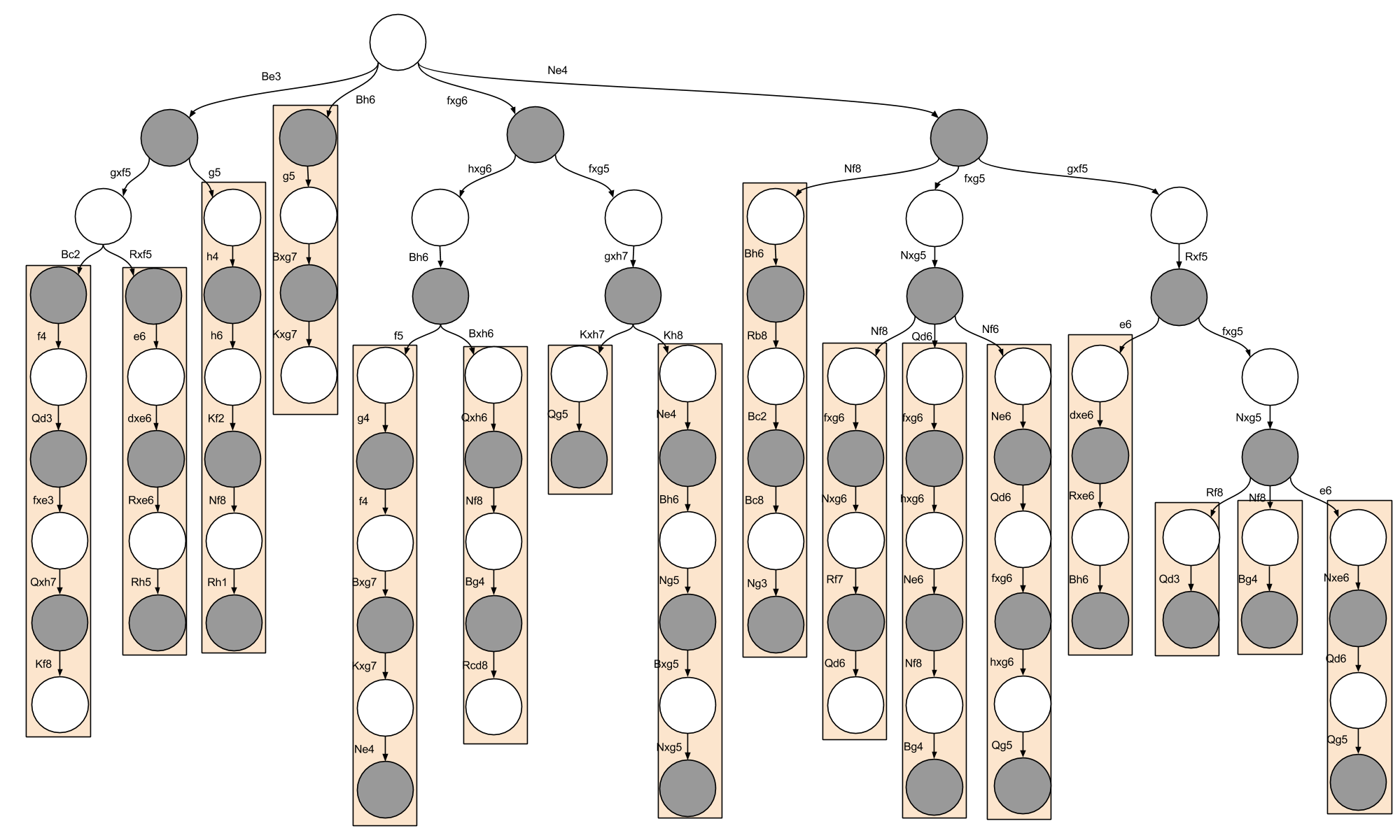
Back to the position at hand. Black is threatening my Bishop: other things being equal, I should remove it from danger. Where to? Bh4 feels wrong: the Bishop is misplaced. Be3 is a natural retreat. Bh6, offering a trade of Bishops (Bxh6 Qxh6), is also possible.

Our spidey-sense should be tingling here. Can we transcend a retreat, and pursue a more aggressive course of action? Can we create threats of our own, scary enough to dissuade Black from capturing our Bishop? If we captured his pawn (fxg6) could Black afford to capture our bishop? Similarly, what if we simply moved our Knight towards his vulnerable King? (Ne4 fxg5 Nxg5) while losing two points, should be examined because our Knight is about to land in the powerful e6 square, and make Black’s life rather bleak.

Please note, explicitly, the kind of tradeoff we are here considering: position vs material (quality vs quantity). Surrendering the latter for the former brings with it a large amount of risk – material factors “persist forever”, whereas positional advantages tend to be fleeting. Further, note that as the pawns are move aside and our pieces make inroads into each others armies, our game will become highly volatile, with the entire game often hinging on one individual moment. When the pace of the game accelerates in this way, it is said to produce sharp positions.

To restate our four options:

22. Be3
22. Bh6
22. fxg6
22. Ne4

I shall now survey my analysis of these options. I spent four hours combing over the implications of these options. I want you to pay attention to the language I use, and the inter-analysis differences you can spot. I will be drawing from such observations in my next post.

Analyzing “Quiet” Moves

For our first positional option, if I play the quiet 22. Be3, Black will most likely resolve the f5-g6 pawn tension:

Suppose Black plays 22 … gxf5.

Here, White cannot play the aggressive 23. Bc2 f4 24. Qd3 because Black’s King escapes after 24 …fxe3 25. Qxh7+ Kf8 (-3.0, [pos 1a]).

Perhaps White does best with the quiet 23. Rxf5 e6 24. dxe6 Rxe6 25. Rh5 with control of the light squares (+0.2, [pos 1b]).

If he instead locks down the Kingside with 22 … g5, I will perhaps want to open it up with 22. h4. Play may proceed 22 …h6 23. Kf2 Nf8 24. Rh1, with play on the Kingside (+0.5, [pos 1c]).

For our second positional option, 22. Bh6 is very similar to Be3, but forces the trade of the dark Bishops.

After 22 …g5 23. Bxg7 Kxg7 Black has more room to breathe than the former line, and can swing his Rooks over to the King’s defense (-0.2, [pos 2a]).

Here are the final positions & scores of the four lines we considered here:

We can represent these analyses graphically, as follows:

We are now done with half of our analysis. Take a deep breath, get a glass of water. We’re almost there! 😛

Analyzing “Sharp” Moves

Consider our first tactical option, 22. fxg6. Black may “play my game” and accept the pawn trade, or “call my bluff” and annihilate my bishop.

On 22 … hxg6 White’s threat is dissolved and he must bring his bishop to safety. After 23. Bh6, Black may try to protect his king by gaining space, or by holing up:

On 23 … f5 White must hammer on Black’s new center before it becomes too strong. 24. g4 can only be met with 24 … f4, after which 25. Bxg7 Kxg7 Ne4 and White’s attack is dead, and is left down a pawn (-0.8, [pos 3a])

Black may instead try the defensive 23 … Bxh6 24. Qxh6 Nf8, but White has a fighting chance after 25. Bg4 Rcd8 where his bishop has a promising view of the light squares (+0.0, [pos 3b])

On 22 … fxg5, Black dares White to prove his attack is worth more than the sacrificed Bishop. White is obliged to blow away Black’s safety net with 23. gxh7, after which Black has two options:

If Black recaptures 23 … Kxh7, after 24. Qxg5 White has a strong attack, potentially leveraging his Re4 to Rh4 (+1.4, [pos 3c])

Black can “hide behind” White’s pawn with 23 … Kh8. A plausible line here may be 24. Ne4 Bh6 25. Ng5 Bxg5 Qxg5, where again White dreams of bringing other pieces to bear in the attack (+0.8, [pos 3d])

Consider instead the second tactical option 22. Ne4. Here, Black may play defensively, capture my bishop, or capture my pawn:

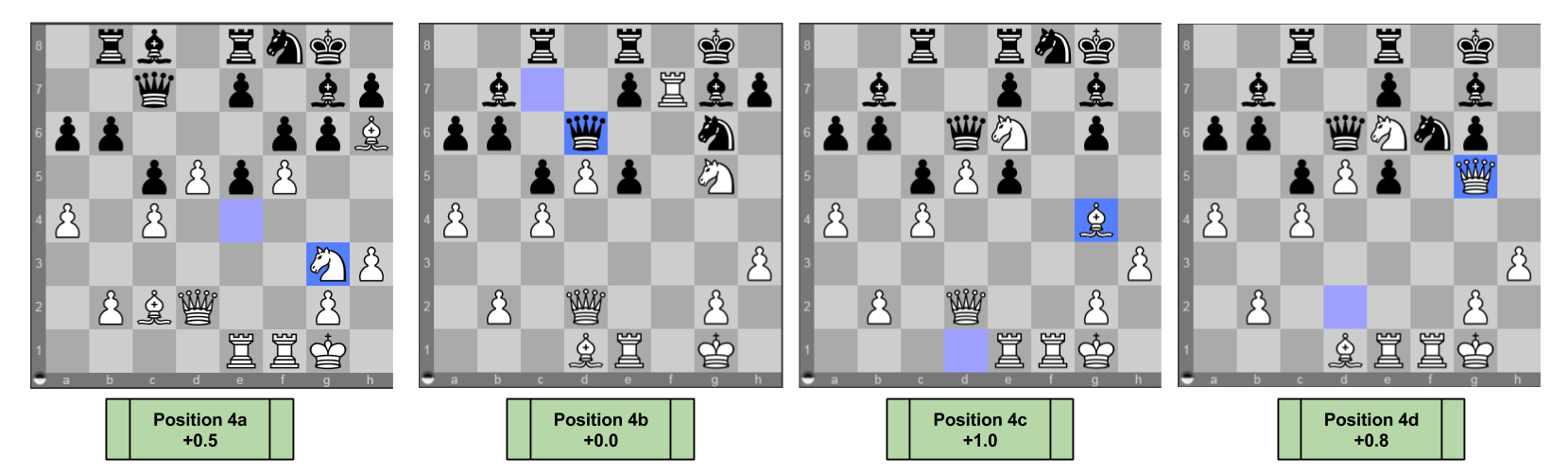
On 22 … Nf8 a plausible line may proceed: 23. Bh6 Rb8 24. Bc2 Bc8 25. Ng3 with strong positional pressure (+0.5, [pos 4a])

On 22 … fxg5 23. Nxg5 Black is faced with several defensive options, of which three stand out:

On 23 … Nf8 24. fxg6 Nxg6 25. Rf7 Black can avoid the Ne6 fork with 25 … Qd6, with a very sharp, unclear game ahead (+0.0, [pos 4b])

On 23 … Qd6 24. fxg6 hxg6 25. Ne6 White’s control of the light squares is very powerful. Play might continue 25 … Nf8 26. Bg4 (+1.0, [pos 4c])

On 23 … Nf6 24. Ne6 Qd6 25. fxg6 hxg6 26. Qg5 White’s Queen bears down on the weak g-file (+0.8, [pos 4d])

On 22 … gxf5 23. Rxf5 Black can challenge the Rook with 23 … e6 after which 24. dxe6 Rxe6. 25. Bh6 and White is comfortable (+1.0, [pos 4e])

But Black can simply capture the bishop on instead. After 23 … fxg5 24. Nxg5, Black is again faced with many defensive options.

On 24 … Rf8 Qd3 White threatens to move the rook and checkmate via Qh7. (+0.9, [pos 4f])

On 24 … Nf8 Bg4 White is poised to threaten the Rc8, and counter Black moving his e-pawn (+0.7, [pos 4g])

On 24 … e6 Nxe6 25. Qd6 Qg5 White threatens Qg7 checkmate, but this threat can be blocked (+0.5, [pos 4h])

We can again represent the above analyses graphically, as follows:

Chess Decisions Are Graph Computations

Congratulations on surviving the past two sections! We’re almost done. Take a deep breath.

The last question on our plate today is:

How should we take the above analyses and produce a move?

This seems difficult to answer. But consider the following simpler question

What is the score of our original four choices?

If we knew the score attached to our four possible moves, we would have an answer: make the move with the best possible score! 🙂

How to solve this simplified question? If we need scores in the head of the tree, graphically our task becomes propagating the already-known leaf scores back up the tree. Let’s see this in action.

We have a clear understanding of the score for the position after 22. Bh6: it is -0.2.

But what is the score after 22. Be3?

To answer this, we must first evaluate the score after 22 … gxf5. It is White’s turn, should he choose 23. Bc2 or 23. Rxf5? He should choose Rxf5, because it has a higher score! In mathematical terms, we simply take the maximum of all white moves: max(0.2, -3.0) = 0.2!

Now that we know that the state after gxf5 is +0.2, what is the score made by Be3? It is Black’s turn, should he choose gxf5 or g5? He should choose gxf5, becuase it has a lower score! In mathematical terms, we simply take the minimum of all of black’s option scores: min(0.2, 0.5) = 0.2

The above two paragraphs express the basics of the minimax algorithm. The name comes from the application of max() for White and min() for Black. Its procedure is how computers, and as I will argue brains, do chess.

Can you apply the same logic to fxg6 and Ne4? Take a moment to valuate their scores, and then come back to check your work!

Be3: 0.2
Bh6: -0.2
fxg6: 0.0
Ne4: 0.0

Now, given these scores for White’s candidate moves, which should White pick? The maximum, or 22. Be3. And that is precisely the move I chose. 🙂

Here’s a graphical representation of the above results:

It is my hope that chess decisions now remind you of lightning physics:

Takeaways

When considering possible moves, it is helpful to graph moves as nodes in a decision tree.
Analyzing chess is hard work!
When you are done constructing the decision tree, the minimax algorithm translates its data into a decision.

Appendix

If anybody is interested in how the game concluded, let me attach a link to it here for completeness. While I did win, I feel like the win was not particularly instructive. This particular moment analyzed above, however, contained a nice mix of different strategies and thereby was pedagogically useful.

1. d4 Nf6 2. c4 g6 3. Nc3 Bg7 4. e4 d6 5. Nf3 O-O 6. Be2 c5 7. d5 a6 8. a4 Nbd7 9. O-O b6 10. h3 Bb7 11. Bf4 Re8 12. Qd2 Qc7 13. Rae1 Rad8 14. Bd3 Nh5 15. Bg5 Ne5 16. Be2 Nxf3+ 17. Bxf3 Nf6 18. Bd1 Rc8 19. f4 Nd7 20. e5 dxe5 21. f5 f6 22. Be3 g5 23. b3 Rb8 24. h4 gxh4 25. Qf2 h3 26. Qg3 Kh8 27. Bh5 hxg2 28. Kxg2 Rg8 29. Bg6 Bh6 30. Rh1 Nf8 31. Rxh6 e6 32. Qh4 exf5 33. Qxf6+ Rg7 34. Kf2 Nxg6 35. Rxg6 hxg6 36. Bh6 Kg8 37. Bxg7 Qxg7 38. Qe6+ Qf7 39. Qxe5 Rf8 40. Qe6 Qxe6 41. Rxe6 Kg7 42. Rxb6 Rf7 43. b4 cxb4 44. Rxb4 Kf6 45. Rb6+ Kg5 46. c5 f4 47. Ne4+ Kh4 48. Nd6 Bxd5 49. Nxf7 Bxf7 50. c6 Be6 51. c7 Bf5 52. Rxg6 Kh5 53. Rg8 1-0

Average Causal Effect

January 21, 2015March 21, 2017kevinbinz 1 Comment

Followup To: Potential Outcome Models
Part Of: Causal Inference sequence
Content Summary: 900 words, 9 min read

Recap

Our takeaways from last time:

Questions of causality have interesting links to “what if” questions (counterfactuals)
We can construct a Possible Outcomes model that deploys counterfactual reasoning to explain observed effects
If we reverse the direction of a Possible Outcomes model, we see that observed reality only partially determines our counterfactual knowledge.
If we look carefully at the relationship between observed variables and their counterfactual implications, we can begin to see a pattern.

Today, we will connect our Possible Outcomes Model back to causality. But first, we must address questions of scale!

Scaling Up Potential Outcome Models

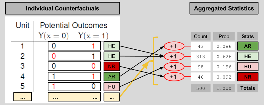
In order to get a sense for the performance of the drug as a whole, one needs to view its effects on a larger population. The above table has N=5 subjects. Let’s imagine 500 subjects instead. Fortunately, if we don’t want to deal with 500 row tables, we can aggregate the data into a shorter entry. Here’s one possible way to compress a large counterfactuals table into four entries:

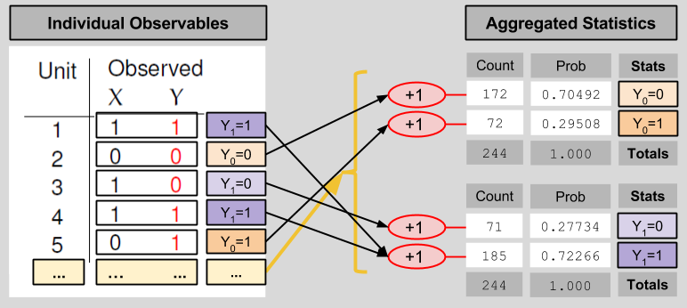
We compress the observables table in an analogous manner:

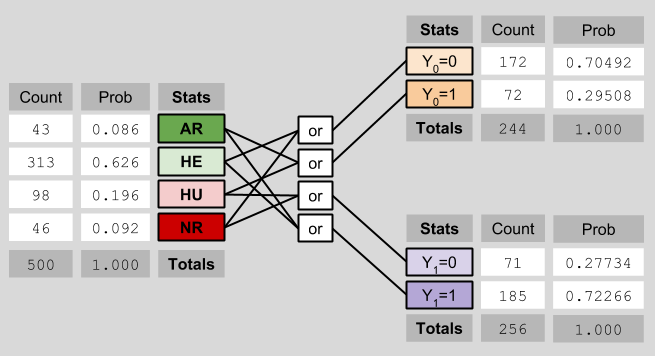
These statistical results relate to each other in the following way:

Average Causal Effect

Let us now shift our gaze from machinery to our original motivation. How might we use potential outcome models to estimate causal effect? If most of our patients are of type NR or AR (Never/Almost Recover), that would suggest that our drug is exerting negligible causal muscle over the patients. However, a drug that indexes many patients of type HE (Helped) seems to have an effect. Conversely, a drug that creates many HU (Hurt) patients can also be said to have a medical impact. Let us create one measure to index both; let Individual Causal Effect (ICE) represent:

ICE = Y₁ – Y₀

Another way of putting the above paragraph, then, is that causally-interesting patients are those with a non-zero ICE score.

As we scale up our model, our causal measure must follow suit. Let Average Causal Effect (ACE) represent:

ACE = P(HE) – P(HU)

In our case (see the diagram about ICE), the ACE = 0.626 – 0.196 = 0.43.

Learning ACE Bounds

Let’s put on our Learning Mode Glasses, and recall that we are unable to observe P(HE) nor P(HU). Instead, we can only view X and Y. What can we learn about the ACE in this context? It is tempting to say “nothing”, since we cannot uniquely determine the counts of the four outcome types. But this would be a mistake, for we can in fact establish bounds for our ACE.

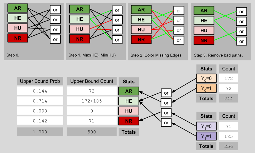
The lower bound of the ACE occurs when the maximum possible number of observed outcomes are ascribed to Hurt people, and the minimum possible number of observed outcomes are ascribed to Helped people:

Thus, the lowest possible value of the ACE is 0.000 – 0.286 = -0.286.

Analogously, the upper bound of the ACE is determinable by imagining a scenario with as few Hurt people, and as many Helped people, as possible:

The highest possible value of the ACE is therefore 0.714 – 0.000 = 0.714. Thus, we can see that (despite not knowing the true ACE), we have shrunk its possible values from [-1, 1] to [-0.286, 0.714]. Importantly, this smaller fence still contains the true ACE of 0.43.

Transcending ACE Bounds

Can we do better than this? Yes. Let us recall an axiom we used to build our Potential Outcomes Framework:

Consistency Principle: Y = Y₁* X + Y₀*(1-X)

This principle is saying nothing more than that the red numbers on our potential models diagrams must match:

It turns out that, if you are willing to purchase an assumptions, you can estimate the true ACE from observed data alone.

Randomization Assumption: selection variable X is independent of the counterfactual table (X ⊥ Y₀, Y₁)

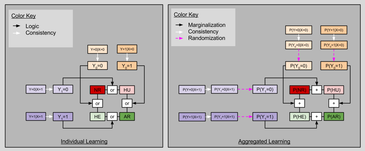
If the Randomization Assumption is true, then we may derive the following startling fact:

P(Y=i|X=1)

= P(Y₁=i|X=1) # Because of Consistency Principle

= P(Y₁=i) # Because of Randomization (X ⊥ Y₁)

= P(Y₁=i, Y₀=1) + P(Y₁=i, Y₀=0) # Marginalization over Y₀

When i=0, we have P(Y₁=0) = P(HU)+ P(NR). When i=1, we have P(Y₁=1) = P(HU)+ P(NR)

By the same logic, we can condition on X=0:

P(Y=i|X=0)

= P(Y₀=i|X=0) # Because of Consistency Principle

= P(Y₀=i) # Because of Randomization (X ⊥ Y₀)

= P(Y₀=i, Y₁=1) + P(Y₀=i, Y₁=0) # Marginalization over Y₁

When i=0, we have P(Y₀=0) = P(HE)+ P(NR). When i=1, we have P(Y₀=1) = P(AR)+ P(HU)

These four facts together exhibit startling similarities to one of our results from last time:

Notice that, although we can never uniquely determine say P(HU) from observables alone, we can estimate the ACE directly!

P(ACE)

= P(HE) – P(HU)

= P(HE) + P(AR) – [P(HU) + P(AR)]

= P(Y₁=1) – P(Y₀=1)

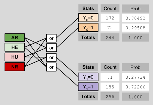
Let’s see this in action. Recall our original data, reproduced in aggregated form below:

Notice that I have explicitly removed the counterfactual data previously visible on the left side of the diagram. This deletion reflects the fact that counterfactual data is intrinsically opaque to us. This depressing fact is known as the Fundamental Problem Of Causal Inference.

Here, we can estimate the ACE as follows:

P(Y₁=1) – P(Y₀=1)

= 0.72266 – 0.29508

= 0.427528

If that’s not close to the ACE true value of 0.43, I don’t know what is. 🙂

Takeaways

Data aggregation statistics are a useful way of summarizing large counterfactual/observable tables.
Rubin’s potential outcome model informs philosophical questions of causality through his Average Causal Effect (ACE) measure
In real-world scenarios, where counterfactual data is opaque to us, we can still derive upper and lower bounds for the ACE
If we are willing to assert the independence of sampling processes, however, we are able to estimate the ACE directly!

Potential Outcome Models

January 19, 2015March 21, 2017kevinbinz Leave a comment

Part Of: Causal Inference sequence
Content Summary: 800 words, 8 min reading time

Counterfactuals

Imagine you are a doctor investigating the effects of a new drug for cancer treatment:

A large number of patients enroll in the trial.
For each patient, you may administer the drug, or a placebo.
For each patient, you record whether the outcome is death or survival (cancer remission).

Let’s sharpen the above account by defining variables across it:

N patients enroll in the trial.
Let X represent applied treatment. Placebo application is X=0; drug application is X=1.
Let Y represent patient outcome. Patient death is Y=0; patient survival is Y=1.

How many patients should we give the drug to? If we give the placebos to all patients, and all of them die, does that mean that our drug works? Of course not! Next, consider the situation where we give the drug to all patients, and all of them live. May we now conclude that the drug is effective in this scenario? Not necessarily: perhaps we have simply encountered a particularly lucky group of human beings.

Imagine next a world where we could acquire answers to any question we dare ask. Here, how would you go about determining the causal effect of our drug?

If a patient dies via the placebo, wouldn’t it be nice if we could rewind time, and observe whether the drug saved their lives (see whether the drug helps this individual)? If a patient dies via the drug, wouldn’t it be nice if we could rewind time and see whether they die via the placebo (perhaps they are beyond help)? In an ideal world, we could rewind time and acquire answers to such what if questions.

For formal name for what-if models of causality are known as counterfactuals. And counterfactual theories of causation are just one location is a vast, turbulent landscape of the West’s struggle over causation. The first time I wandered into Wikipedia’s survey of causal reasoning, my head was throbbing for hours. But let me spare you an attempt to make sense out of the philosophical implications of counterfactuals, and merely paint a formalism.

An Outcome Taxonomy

We require two more variables:

Let Y₀ represent patient outcome after placebo administration. Thus, Y₀=1 means placebo patient lives.
Let Y₁ represent patient outcome after drug administration. Thus, Y₁=0 means drugged patient dies.

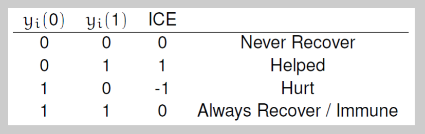
There are only four possible types of patient:

Translating back into English:

Patients of type “Never Recover” will die if given the drug, but will also die if given a placebo.
Patients of type “Helped” will survive if given the drug, but will die if given a placebo.
Patients of type “Hurt” will die if given the drug, but will live if given a placebo.
Patients of type “Always Recover” will live if given the drug, but will also live if given a placebo.

The Machinery Of Possibility

Imagine you are omniscient, and have access to a counterfactual table of possible outcomes. That is, for either possible world (the one where you hand me a drug, and the one where you hand me a placebo), you know whether I beat my cancer. You can then generate predictions as follows:

The left table is one of counterfactuals, the right is composed of observables. The X column represents a selector; it selects which column of the counterfactual table from which to draw the value of Y (X=1 means right column, X=0 means left). Pay attention to the color red, until the above makes sense.

Now let’s relax the problem and admit that we are not omniscient: scientists simply do not possess privileged access to the multiverse. Rather, you simply observe outcomes of individuals. In this world, inference moves from right-to-left, and half of all counterfactual entries are left indeterminate.

As you can see, these indeterminate counterfactuals on the left means that the patient of that row is of indeterminate type. If a patient dies after using the placebo (second row), we do not know whether she would Never Recover, or if she would have been Helped by the drug!

Mechanized Outcome Constraint

Pay attention to the color patterns in the above image. Could you have predicted that particular pattern? I couldn’t; they feel mysterious.

If you notice your confusion, you are more likely to expend effort to dissolve it. Patterns emerge after the following process:

Please take a minute to come to terms with the above diagram. Do you see how each step flows from the previous? If not, please comment!

After the final step, we notice a nice symmetry between counterfactual results.

Takeaways

Questions of causality have interesting links to “what if” questions (counterfactuals)
We can construct a Possible Outcomes model that deploys counterfactual reasoning to explain observed effects
If we reverse the direction of a Possible Outcomes model, we see that observed reality only partially determines our counterfactual knowledge.
If we look carefully at the relationship between observed variables and their counterfactual implications, we can begin to see a pattern.

Next time, we will exploit the symmetry above to complete our picture of potential-outcome causality. See you then!

[Excerpt] The Hiccups Of Your Inner Fish

January 19, 2015June 4, 2019kevinbinz Leave a comment

Excerpt From: Your Inner Fish
Content Summary: 1000 words, 5 min read

The annoyance of hiccups has its roots in the history we share with fish and tadpoles.

If there is any consolation for getting hiccups, it is that our misery is shared with many other mammals. Cats can be stimulated to hiccup by sending an electrical impulse to a small patch of tissue in their brain stem. This area of the brain stem is thought to be the center that controls the complicated reflex that we call a hiccup.

The hiccup reflex is a stereotyped twitch involving a number of muscles in our body wall, diaphragm, neck, and throat. A spasm in one or two of the major nerves that control breathing causes these muscles to contract. This results in a very sharp inspiration of air. Then, about 35 milliseconds later, a flap of tissue in the back of our throat (the glottis) closes the top of our airway. The fast inhalation followed by a brief closure of the tube produces the “hic”.

The problem is that we rarely experience only a single hic. Stop the hiccups in the first five to ten hics, and you have a decent chance of ending the bout altogether. Miss that window, and the bout of hiccups can persist for an average of about sixty hics. Inhaling carbon dioxide (by breathing into the classic paper bag) and stretching the body wall (taking a big inhalation and holding it) can end hiccups early in some of us. But not all. Some cases of pathological hiccups can be extremely prolonged. The longest uninterrupted hiccups in a person lasted from 1922 to 1990.

Our tendency to develop hiccups is another influence of our past. There are two issues to think about:

What causes the spasm of nerves that initiates the hiccup.
What controls the distinctive hic, the abrupt inhalation-glottis closure.

The nerve spasm is a product of our fish history, while the hic is an outcome of the history we share with animals such as tadpoles.

First, fish. Our brain can control our breathing without needing conscious effort on our part. Most of the work takes place in the brain stem, at the boundary between the brain and the spinal cord. The brain stem sends nerve impulses to our main breathing muscles. Breathing happens in a pattern. Muscles of the chest, diaphragm, and throat contract in a well-defined order. Consequently, this part of the brain stem is known as a “central pattern generator.” This region can produce rhythmic patterns of nerve and, consequently, muscle activation. A number of such generators in our brain and spinal cord control other rhythmic behaviors, such as swallowing and walking.

The problem is that the brain stem originally controlled breathing in fish; it has been jury-rigged to work in mammals. Sharks and bony fish all have a portion of the brain stem that controls the rhythmic firing of muscles in the throat and around the gills. The nerves that control these areas all originate in a well-defined portion of the brain stem. We can even see this nerve arrangement in some of the most primitive fish in the fossil record. Ancient ostracoderms, from rocks over 400 million years old, preserve casts of the brain and cranial nerves. Just as in living fish, the nerves that control breathing extend from the brain stem.

This works well in fish, but it is a lousy arrangement for mammals. In fish, the nerves that control breathing do not have to travel very far from the brain stem. The gills and throat generally surround this area of the brain. We mammals have a different problem. Our breathing is controlled by muscles in the wall of our chest and by the diaphragm, the sheet of muscle that separates our chest from our abdomen. Contraction of the diaphragm controls inspiration. The nerves that control the diaphragm exit our brain just as they do in fish, and they leave from the brain stem, near our neck. These nerves, the vagus and the phrenic nerve, extend from the base of the skull and travel through the chest cavity and reach the diaphragm and the portions of the chest that control breathing. This convoluted path creates problems; a rational design would have the nerves traveling not from the neck but from nearer the diaphragm. Unfortunately, anything that interferes with one of these nerves can block their function or cause a spasm.

If the odd course of our nerves is a product of our fishy past, the hiccup itself is likely the product of our history as amphibians. Hiccups are unique among our breathing behaviors in that an abrupt intake of air is followed by a closure of the glottis. Hiccups seem to be controlled by a central pattern generator in the brain stem: stimulate this region with an electrical impulse, and we stimulate hiccups. It makes sense that hiccups are controlled by a central pattern generator, since, as in other rhythmic behaviors, a set sequence of events happens during a hic.

It turns out that the pattern generator responsible for hiccups is virtually identical to one in amphibians. And not in just amphibians – in tadpoles, which use both lungs and gills to breathe. Tadpoles use this pattern generator when they breathe with gills. In that circumstance, they want to pump water into their mouth and throat and across the gills, but they do not want the water to enter their lungs. To prevent it from doing so, they close the glottis, the flap that closes off the breathing tube. And to close the glottis, tadpoles have a central pattern generator in their brain stem so that an inspiration is followed immediately by a closing glottis. They can breathe with their gills thanks to an extended form of hiccup.

The parallels between our hiccups and gill breathing in tadpoles are so extensive that many have proposed that the two phenomena are one and the same. Gill breathing in tadpoles can be blocked by carbon dioxide, just like our hiccups. We can also block gill breathing by stretching the wall of the chest, just as we can stop hiccups by inhaling deeply and holding our breath. Perhaps we could even block gill breathing in tadpoles by having them drink a glass of water upside down.

The Categorical Simplex

January 10, 2015March 27, 2017kevinbinz Leave a comment

Part Of: Probability Theory sequence
Content Summary: 1000 words, 10 min read

Describing Depression

In An Introduction To Bayesian Inference, you were introduced to the discrete random variable:

You remember algebra, and how annoying it was to use symbols that merely represented numbers? Statisticians get their jollies by terrorizing people with a similar toy, the random variable. The set of all possible values for a given variable is known as its domain.

Let’s define a discrete random variable called Happy. We are now in a position to evaluate expressions like Probability(Happy=true)

The domain of Happy is of size two (it can resolve to either true, or false). Since domain size is pivotal in this post, we will abbreviate it. Let an Variable_N be a discrete random variable whose domain is size N (in the literature, the probability distribution for Variable_Nis known as the categorical distribution).

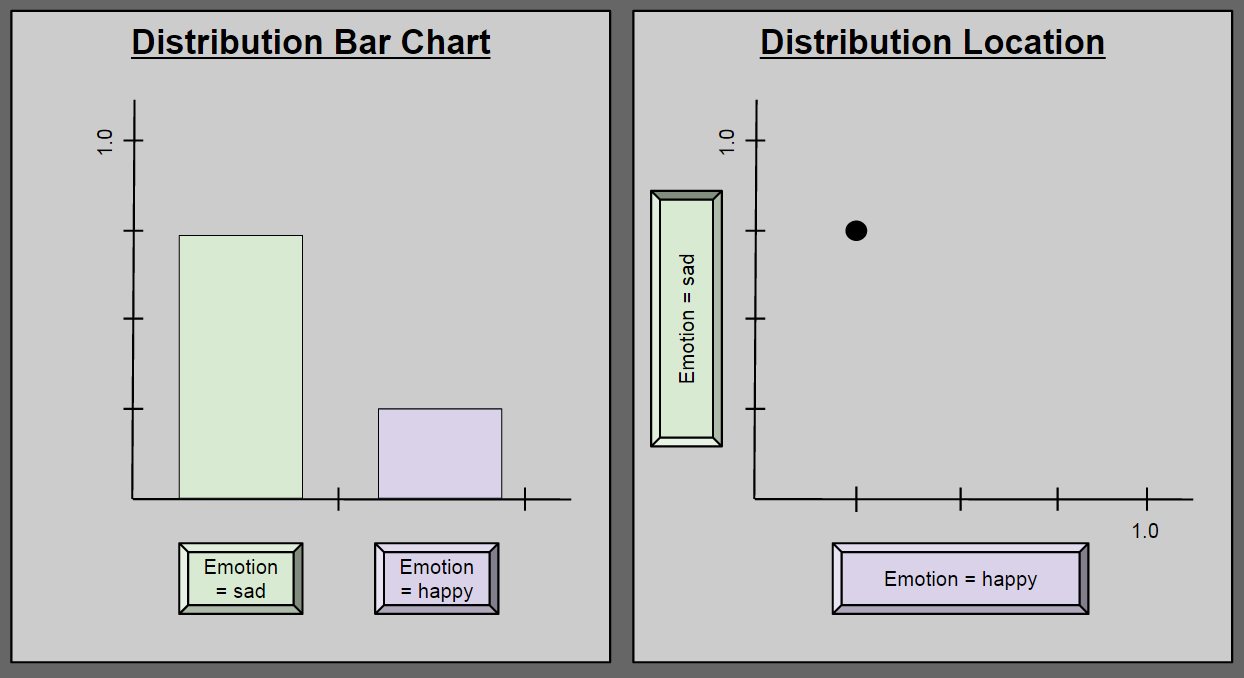
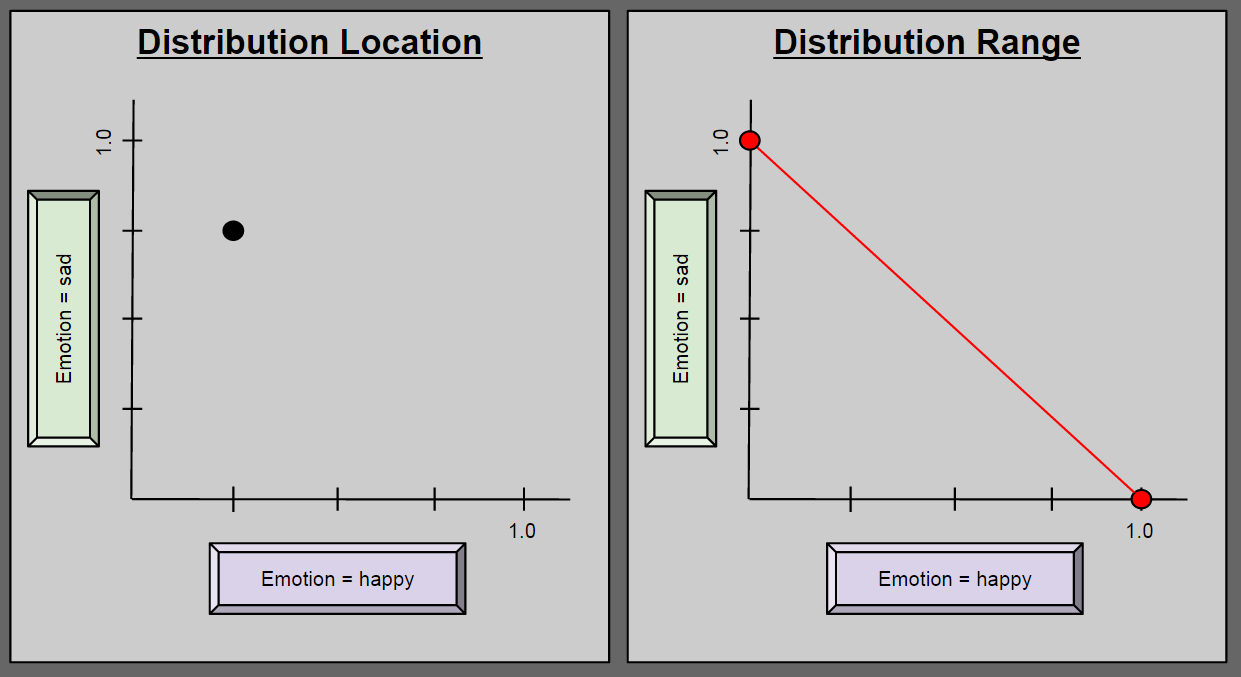
Consider a new variable, Emotion₂ = { happy, sad }. Suppose we use this variable to describe a person undergoing a major depression. At any one time, such a person may have a 25% chance of being happy, and a 75% chance of being sad. This state of affairs can be described in two ways:

Pause here until you can explain to yourself why these diagrams are equivalent.

A Modest Explanation Of All Emotion

We have seen how a particular configuration of Emotion₂can accurately characterize a depressed person. But Emotion₂is intended to describe all possible human emotion. Can it take on any value in this two-dimensional space? No: to describe a human being as P(happy) = 1.5; P(sad) = -0.1 is nonsensical. So what values besides (0.25, 0.75) are possible for Emotion₂?

The above range diagram (right side) answers our question: any instance of Emotion₂ must reside along the red line. Take a second to convince yourself of this. It sometimes helps to think about the endpoints (0.0, 1.0) and (1.0, 0.0).

Bar Charts Are Hyperlocations

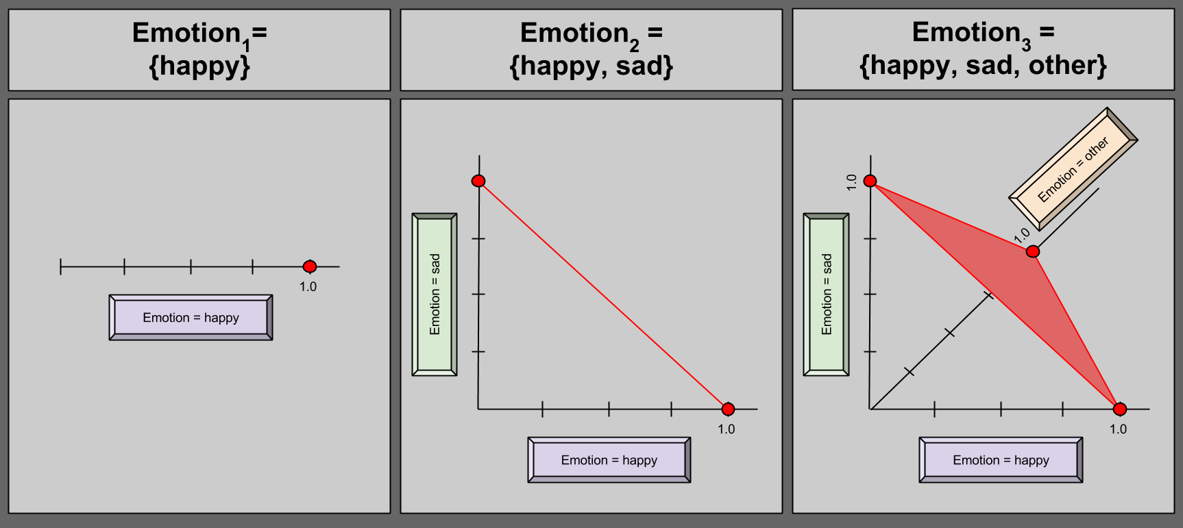
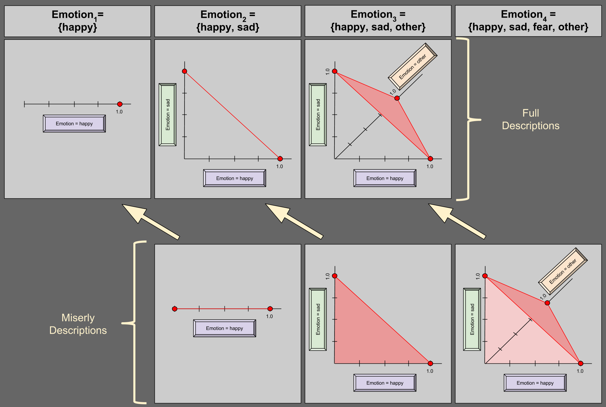
Perhaps you are not enthralled with the descriptive power of Emotion₂. Perhaps you subscribe to the heresy that certain human experiences cannot be usefully described as either happy or sad. Let us expand our model to catch these “corner cases”, and define Emotion₃ = { happy, sad, other }.

Can we identify a distribution range of this new variable? Of course!

Take a moment to convince yourself that Emotion₃ may never contain any point outside the shaded red area.

Alright, so we have a fairly pleasing geometric picture of a discrete random variables with domains up to size 3. But what happens when we mature our model again? Imagine expanding our random variable to encapsulate the six universal emotions.

Could you draw a bar chart for an arbitrary Emotion₆?

Of course you could; you’d simply need to add four more bars to the first diagram of this post.

Now, what about location in space?

Drawing in 6-D is hard. 🙂

Here is the paradox: a simple bar chart corresponds with a cognitively intractable point in 6-dimensional space. I hope you never look at bar charts the same way!

An aside that, despite the constant three being sloppily hardcoded into our mental software, it turns out that reasoning about hyperlocations – points in N-dimensional space – is an important conceptual tool. If I ever get around to summarizing Drescher’s Good and Real, you’ll see hyperlocations used to establish an intuitive guide to quantum mechanics!

Miserly Description

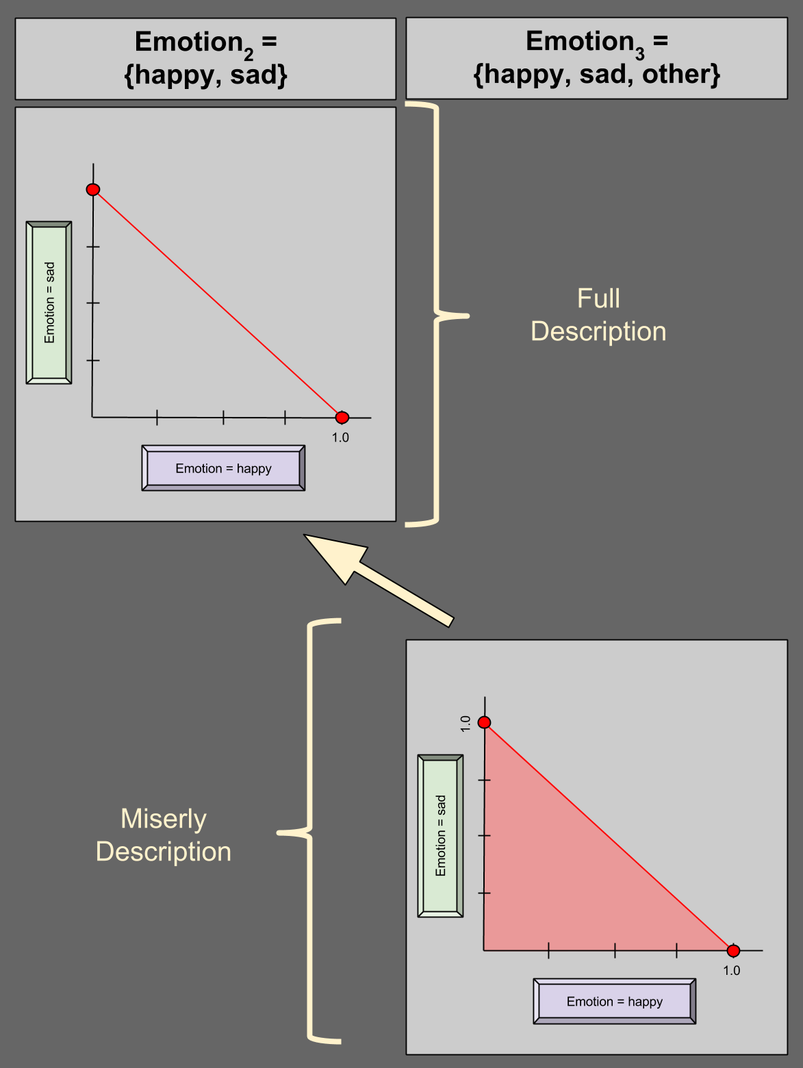
But do we really need 6-dimensional space to describe a domain of size 6? Perhaps surprisingly, we do not. Consider the case of Emotion₃ = {happy, sad, other} again. Suppose I give you P(happy) = 0.5; P(sad) = 0.2. Do you really need me to tell you the P(other) = 0.3?

You could figure this out on your own, because the remaining 30% has to come from somewhere (0.3 = 1.0 – 0.5 – 0.2).

Given this fact that a variable has a 100% chance of being something (aka unitarity), we can describe a 4-variable in 3 dimensions:

In the bottom-right of the diagram, we see an illustration of miserly description. Suppose we are given (0.25, 0.25) for happy and sad, respectively. P(other) must then be valued at 0.5, and (0.25, 0.25) is thus a valid distribution – this is confirmed by its residence in the shaded region above. Suppose I give you any point on the dark red edge of the region (e.g., (1.0, 0.0)); what value for P(other) must you expect? Zero.

This generalizes: unitarity allows us to describe an N-variable in N-1 dimensions. Here are two more examples:

Notice the geometric similarities between the two descriptive styles, denoted by the yellow arrows.

The Hypervolume Of Probability

Consider the bottom row of our last figure (miserly descriptions). These geometric objects look similar: a triangle is not very different from a tetrahedron. What happens when we again move into a higher-dimensional space? Well, it turns out that there’s a name for this shape: a simplex is a generalization of a triangle into arbitrary dimensions. Personally, I would have preferred the term “hyperpyramid”, but I suppose the book of history is shut on this topic. 😛

We have thus arrived at an important result. The probability distribution associated with a discrete random variable can be represented as a simplex.

A Link To Convexity

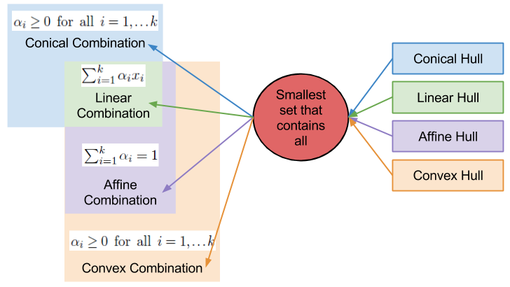
I want you to recall my discussion on convex combinations.

A convex combination should smell a lot like a probability distribution. Consider the axioms of Kolmogorov’s probability theory:

The probability of an event is a non-negative real number.
The probability that some event in the entire sample space will occur is 1.0
The probability of the intersection of several events is equal to the sum of their individual probabilities.

If you compare these axioms to the maths of the above combinations, and squint a little, you’ll begin to hypothesize similarities. 🙂

It turns out simplices form a bridge between convex hulls and probability distributions, because a simplex simply is a convex hull.

Takeaways

Discrete random variables can refer to domains with more than two events.
As a description, a bar chart is interchangeable with a hyperlocation.
The range of possible probability distributions is relatively easy to characterize
We can describe one fewer dimension of a distribution by leveraging the fact of unitarity.
Such “miserly descriptions” reveal that all possible probability distributions of a categorical random variable is a generalized triangle (a simplex).
This geometric result reveals a deep connection between the foundations of probability theory and convex analysis.