Part Of:Optimization sequence Content Summary: 800 words, 8 min read.
Today, I introduce the concept of duality. Buckle your seat belts! 🙂
Max Flow algorithm
The problem of flow was originally studied in the context of the USSR railway system in the 1930s. The Russian mathematician A.N. Tolstoy published his Methods of finding the minimal total kilometrage in cargo-transportation planning in space, where he formalized the problem as follows.
We interpret transportation graphically. Vertices are interpreted as cities, and edges are railroads connecting two cities. The capacity of each edge was the amount of goods that particular railroad could transport in a given day. The bottleneck is solely the capacities, and not production and consumption. We assume no available storage at the intermediate cities.
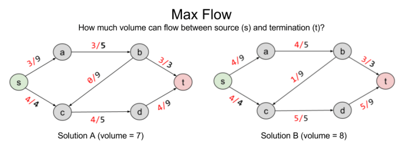
The flow allocation problem defines source and termination vertices, s and t. We desire to maximize volume of goods transported s → t. To do this, we label each edge with the amount of goods we intend to ship on that railroad. This quantity, which we will call flow, must respect the following properties:
Flow cannot exceed the capacity of the railroad.
Flow is conserved: stuff leaving a city must equal the amount of stuff arriving.
Here are two possible solutions to flow allocation:
Solution B improves on A by pushing volume onto the b → c railway. But are there better solutions?
To answer rigorously, we formalize max flow as a linear optimization problem:
The solution to LP tells us that no, eight is the maximum possible flow.
Min Cut algorithm
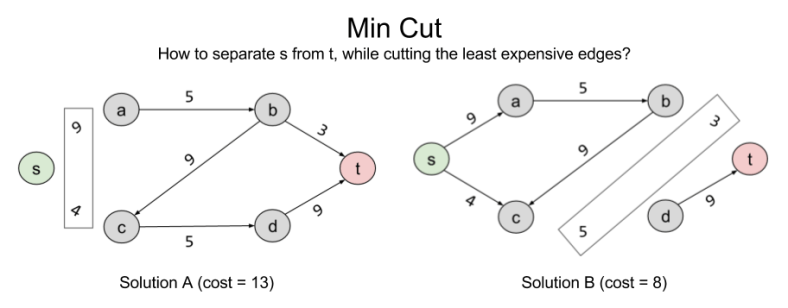
Consider another, seemingly unrelated, problem we might wish to solve: separability. Let X ⊂ E represent the number of edges you need to remove to eliminate a connection s → t. Here are two such solutions:
Can we do better than B? The answer is no: { (b,t), (c,d) } is the minimum cut possible in the current graph. In linear programming terms, it is the Best Feasible Solution (BFS)
Note that the BFS of minimum cut and the BFS of max flow arrive at the same value. 8 = 8. This is not a coincidence. In fact, these problems are intimately related to one another. What the min cut algorithm is searching for is the bottleneck: the smallest section of the “pipe” from s → t. For complex graphs like this, it is not trivial to derive this answer visually; but the separability algorithm does the work for us.
The deep symmetry between max flow and min cut demonstrates an important mathematical fact. All algorithms come in pairs. For this example, we will call max flow and min cut the primal and dual problems, respectively. We will explore the ramifications for this another time. For now, let’s approach duality from an algebraic perspective.
Finding LP Upper Bound
Consider a linear program with the following objective function:
And these constraints
This program wants to find the largest solution possible given constraints. Can we provide an upper bound on the solution?
Yes. We can immediately say that the solution is no greater than 6. Why? The objective function, is always smaller than , because we know all variables are positive. So we have an upper bound OPT ≤ 6. We can sharpen this upper bound, by comparing the objective function to other linear combinations of the constraints.
Different weights to our linear combinations produce different upper bounds:
(1,0) → 6
(0,1) → 5
(⅓, ⅓ ) → 3.67
Let us call these two weights . What values of these variables give us the smallest upper bound? Importantly, this is itself an objective function: .
But and are constrained: they must produce an equation that exceeds . Thus,
and
This gives us our two constraints. Thus, by looking for the lowest upper bound on our primal LP, we have derived our dual LP:
Note the extraordinary symmetry between primal and dual LPs. The purple & orange values are mirror images of one another. Further, the constraint coefficient matrix has transposed (the 3 has swapped along the diagonal). This symmetry is reflected in the above linear algebra formulae.
A Theory of Duality
Recall that linear programs have three possible outcomes: infeasible (no solution exists), unbounded (solution exists at +/-∞) or feasible/optimal. Since constraints are nothing more than geometric half-spaces, these possible outcomes reflect three kinds of polyhedra:
The outcome of primal and dual programs are predictably correlated. Of the nine potential pairings, only four can actually occur:
Both P and D are infeasible
P is unbounded and D is infeasible
D is unbounded and P is infeasible
Both are feasible, and there exist optimal solutions
Finally, in the above examples, we saw that the optimal dual value . But this is not always the case. In fact, the optimal dual value can be smaller .
We can distinguish between two kinds of duality:
Strong duality, where
Weak duality, where
Takeaways
Today, we have illustrated a deep mathematical fact: all problems come in pairs. Next time, we will explore the profound ramifications of this duality principle.
Part Of: Information Theory sequence Content Summary: 900 words, 9 min read
Motivations
What do probabilities mean?
A frequentist believes that they represent frequencies. P(snow) =10% means that on 100 days just like this one, 10 of them will have snow.
A Bayesian, on the other hand, views probability as degree of belief. P(snow) = 10% means that you believe there is a 10% chance it will snow today.
This subjective approach views reasoning as probability (degree of belief) spread over possibility. On this view, Bayes Theorem provides a complete theory of inference:
From this equation, we see how information updates our belief probabilities. Bayesian updating describes this transition from prior to posterior, P(H) → P(H|E).
As evidence accumulates, one’s “belief distributions” tend to become sharply peaked. Here, we see degree of belief in a hockey goalie’s skill, as we observe him play. (Image credit Greater Than Plus Minus):
What does it mean for a distribution to be uncertain? We would like to say that our certainty grows as the distribution sharpens. Unfortunately, probability theory provides no language to quantify this intuition.
This is where information theory comes to the rescue. In 1948 Claude Shannon discovered a unique, unambiguous way to measure probabilistic uncertainty.
What is this function? And how did he discover it? Let’s find out.
Desiderata For An Uncertainty Measure
We desire some quantity H(p) which measures the uncertainty of a distribution.
To derive H, we must specify its desiderata, or what we want it to do. This task may feel daunting. But in fact, very simple conditions already determine H to within a constant factor.
We require H to meet the following conditions:
Continuous. H(p) is a continuous function.
Monotonic. H(p) for an equiprobable distribution (that is, A(n) = H(1/n, 1/n, 1/n)) is a monotonic increasing function of n.
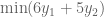
Compositionally Invariant. If we reorganize X by bundling individual outcomes into single variables (b: X → W), H is unchanged, H(X) = H(W).
Let’s explore compositional invariance in more detail.
Deriving H
Let us consider some variable that can assume discrete values . Our partial understanding of the processes which determine are the probabilities . We would like to find some , which measures the uncertainty of this distribution.
Suppose has three possible outcomes. We can derive by combining events x2 and x3.
The uncertainty of must be invariant to such bundling. So we have that:
The right tree has two distributions and . The uncertainty of two distributions is the sum of each individual uncertainty. Thus we add H(⅔, ⅓). But this distribution is reached only ½ of the time, so we multiply by 0.5.
How does composition affect equiprobable distributions ? Consider a new with 12 possible outcomes, each equally likely to occur. The uncertainty , by definition. Suppose we choose to bundle these branches by . Then we have:
But suppose we choose a different bundling function . This simplifies things:
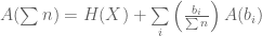
For what function of does hold? There is only one solution, as shown in Shannon’s paper:
varies with logarithmic base (bits, trits, nats, etc). With this solution we can derive a general formula for entropy .
Recall,
← Found by uniform bundling (eg., )
← Found by arbitrary bundling (eg., )
Hence,
We have arrived at our definition of uncertainty, the entropy H(X):
To illustrate, consider a coin with bias p. Our uncertainty is maximized for a fair coin, p = 0.5, and smallest at p = 0.0 (certain tails) or 1.0 (certain heads).
Entropy vs Information
What is the relationship between uncertainty and information? To answer this, we must first understand information.
Consider the number of possible sentences in a book. Is this information? Two books contain exponentially more possible sentences than one book.
When we speak of information, we desire it to scale linearly with its length. Two books should contain approximately twice as much information.
If we take the logarithm of the possible messages , we can preserve this intuition:
Recall that,
From here, we can show that entropy is expected information:
What does this discovery mean, though?
Imagine a device that produces 3 symbols, A, B, or C. As we wait for the next symbol, we are uncertain which symbol comes next. Once a symbol appears our uncertainty decreases, because we have received more information. Information is a decrease in entropy.
If A, B, and C occur at the same frequency, we should not be surprised to see any one letter. But if P(A) approaches 0, then we will be very surprised to see it appear, and the formula says I(X) approaches ∞. For the receiver of a message, information represents surprisal.
On this interpretation, the above formula becomes clear. Uncertainty is anticipated surprise. If our knowledge is incomplete, we expect surprise. But confident knowledge is “surprised by surprise”.
Conclusions
The great contribution of information theory lies in a measure for probabilistic uncertainty.
We desire this measure to be continuous, monotonic, and compositionally invariant. There is only one such function, the entropy H:
This explains why a broad distribution is more uncertain than one that is narrow.
Henceforth, we will view the words “entropy” and “uncertainty” as synonymous.
Related Works
Shannon (1948). A Mathematical Theory of Communication
Jaynes (1957). Information Theory and Statistical Mechanics
Part Of: [Neuroeconomics] sequence Content Summary: 1500 words, 15 min reading time
Preliminaries
Decisions are bridges between perception and action. Not all decisions are cognitive. Instead, they occur at all levels of the abstraction hierarchy, and include things like reflexes.
Theories of decision tend to constrain themselves to cognitive phenomena. They come in two flavors: descriptive (“how does it happen”) and normative (“how should it happen”).
Decision making often occurs in the context of imperfect knowledge. We may use probability theory as a language to reason about uncertainty.
Let risk denote variance in the probability distribution of possible outcomes. Risk can exist regardless of whether a potential loss is involved. For example, a prospect that offers a 50-50 chance of paying $100 or nothing is more risky than a prospect that offers $50 for sure – even though the risky prospect entails no possibility of losing money.
Today, we will explore the history of decision theory, and the emergence of prospect theory. As the cornerstone of behavioral economics, prospect theory provides an important theoretical surface to the emerging discipline of neuroeconomics.
Maximizing Profit with Expected Value
Decision theories date back to the 17th century, and a correspondence between Pascal and Fermat. There, consumers were expected to maximize expected value (EV), which is defined as probability p multiplied by outcome value x.
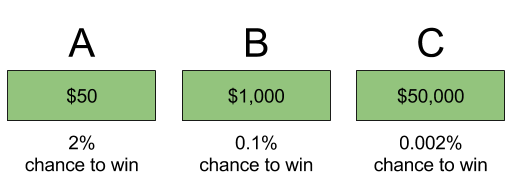
To illustrate, consider the following lottery tickets:
Suppose each ticket costs 50 cents, and you have one million dollars to spend. Crucially, it doesn’t matter which ticket you buy! Each of these tickets has the same expected value: $1. Thus, it doesn’t matter if you spend the million dollars on A, B, or C – each leads to the same amount of profit.
The above tickets have equal expected value, but they do not have equal risk. We call people who prefer choice A risk averse; whereas someone who prefers C is risk seeking.
Introducing Expected Utility
Economic transactions can be difficult to evaluate. When trading an apple for an orange, which is more valuable? That depends on a person’s unique tastes. In other words, value is subjective.
Let utility represent subjective value. We can treat utility as a function u() that operates on objective outcome x. Expected utility, then, is highly analogous to expected value:
Every person’s utility function may be different. If a person’s utility curve is linear, then expected utility converges onto expected value:
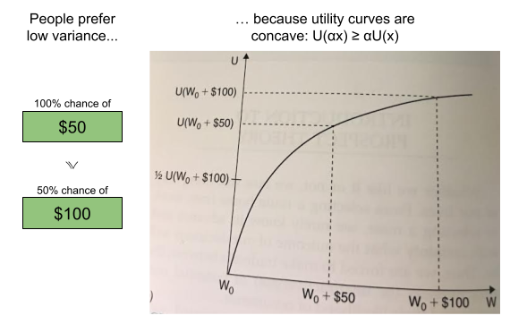
Recall in the above lottery, the behavioral distinction between risk-seeking (preferring ticket A) and risk-averse (preferring C). Well, in practice most people prefer A. Why?
We can explain this behavior by appealing to the shape of the utility curve! Utility concavity produces risk aversion:
In the above, we see the first $50 (first vertical line) produces more utility (first horizontal line) than the second $50.
Intuitively, the first $50 is needed more than the second $50. The larger your wealth, the less your need. This phenomenon is known as diminishing marginal returns.
Neoclassical Economics
In 1944, von Neumann and Morgenstern formulated a set of axioms that are both necessary and sufficient for representing a decision-maker’s choices by the maximization of expected utility.
Specifically, if you assume an agent’s preference set accommodates these axioms…
1. Completeness. People have preferences over all lotteries.
either or or
2. Transitivity. Preferences are expressed consistently.
if and then
3. Continuity. Preferences are expressed as probabilities.
then s.t. iff
4. Substitution. If you prefer (or are indifferent to) lottery over , mixing both with the same third lottery in the same proportion α must not reverse that preference—adding identical “padding” is irrelevant to the choice.
The above axioms constitute expected utility theory, and form the cornerstone for neoclassical economics. Expected utility theory bills itself as botha normative and descriptive theory: that we understand human decision making, and have a language to explain why it is correct.
Challenges To Substitution Axiom
In the 1970s, expected utility theory came under heavy fire for failing to predict human behavior. The emerging school of behavioral economics gathered empirical evidence that von Neumann-Morgenstern axioms were routinely violated in practice, especially the substitution axiom.
For example, the Allais paradox asks our preferences for the following choices:
Most people prefer A (“certain win”) and D (“bigger number”). But these preferences are inconsistent, because C = 0.01A and D = 0.01B. The substitution axiom instead predicts that A ≽ B if and only if C ≽ D.
The Decoy effect contradicts the Independence of Irrelevant Alternatives (IIA). I find it to be best illustrated with popcorn:
Towards a Value Function
Concurrently to these criticisms of the substitution axiom, the heuristics and biases literature (led by Kahneman and Tversky) began to discover new behaviors that demanded explanation:
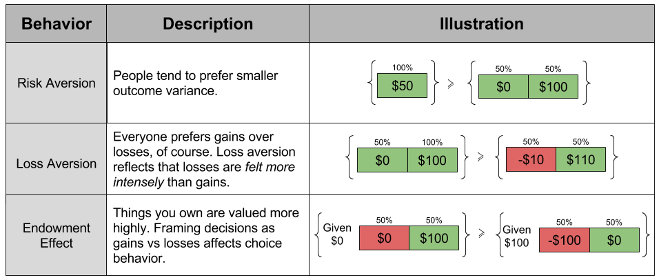
Risk Aversion. In most decisions, people tend to prefer smaller variance in outcomes.
Everyone prefers gains over losses, of course. Loss Aversion reflects that losses are felt more intensely than gains of equal magnitude.
The Endowment Effect. Things you own are intrinsically valued more highly. Framing decisions as gains or as losses affects choice behavior.
Each of these behavioral findings violate the substitution axiom, and cumulatively demanded a new theory. And in 1979, Kahneman and Tversky put forward prospect theory to explain all of the above effects.
Their biggest innovation was to rethink the utility function. Do you recall how neoclassical economics appealed to concavity to explain risk aversion? Prospect theory takes this approach yet further, and seeks to explain all of the above behaviors using a more complex shapeof the utility function.
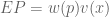
Let value function represent our updated notion of utility. We can define expected prospect of a function as probability multiplied by the value function
Terminology aside, each theory only differs in the shape of its outcome function.
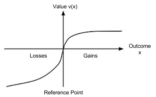
Let us now look closer at the the shape of :
This shape allows us to explain the above behaviors:
The endowment effect captures the fact that we value things we own more highly. The reference point in , where , captures the status quo. Thus, the reference point allows us to differentiate gains and losses, thereby producing the endowment effect.
Loss aversion captures the fact that losses are felt more strongly than gains. The magnitude of is larger in the losses dimension. This asymmetry explains loss aversion.
We have already explained risk aversion by concavity of the utility function . retains concavity for material gains. Thus, we have retained our ability to explain risk aversion in situations of possible gains. For losses, convexity predicts risk seeking.
Towards a Weight Function
Another behavioral discovery, however, immediately put prospect theory in doubt:
The Fourfold Pattern. For situations that involve very high or very low probabilities, participants often switch their approaches to risk.
To be specific, here are the four situations and their resultant behaviors:
Fear of Disappointment. With a 95% chance to win $100, most people are risk averse.
Hope To Avoid Loss. With a 95% chance to lose $100, most people are risk seeking.
Hope Of Large Gain. With a 5% chance to win $100, most people are risk seeking.
Fear of Large Loss. With a 5% chance to lose $100, most people are risk averse.
Crucially, fails to predict this behavior. As we saw in the previous section, it predicts risk aversion for gains, and risk seeking for losses:
Failed predictions are not a death knell to a theory. Under certain conditions, they can inspire a theory to become stronger!
Prospect theory was improved by incorporating a probability-weighting function.
Where has the following shape:
These are in fact two probability-weighting functions (Hertwig & Erev 2009)
Explicit weights represent probabilities learned through language; e.g., when reading the sentence “there is a 5% chance of reward”.
Implicit weights represent probabilities learned through experience, e.g., when the last 5 out of 100 trials yielded a reward.
This change adds some mathematical muscle to the ancient proverb:
Humans don’t handle extreme probabilities well.
And indeed, the explicit probability-weighting function successfully recovers the fourfold pattern:
Takeaways
Today we have reviewed theories of expected value, expected utility (neoclassical economics), and prospect theory. Each theory corresponds to a particular set of conceptual commitments, as well a particular formula:
However, we can unify these into a single value formula V:
In this light, EV and EU have the same structure as prospect theory. Prospect theory distinguishes itself by using empirically motivated shapes:
With these tools, prospect theory successfully recovers a wide swathe of economic behaviors.
Until next time.
Works Cited
Hertwig & Erev (2009). The description–experience gap in risky choice
Today, we turn our gaze to Markov Decision Processes (MDPs), a decision-making environment which supports our propensity to learn from good and bad outcomes. We represent outcome desirability with a single number, R. This value is used to refine action selection: given a particular situation, what action will maximize expected reward?
In biology, we can describe the primary work performed by an organism is to maintain homeostasis: maintaining metabolic energy reserves, body temperature, etc in a widely varying world.
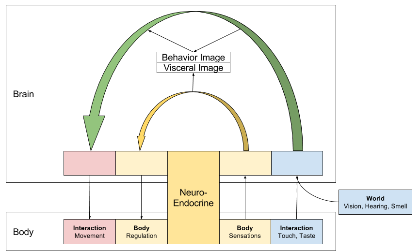
Cybernetics provide a clear way of conceptualizing biological reward. In Neuroendocrine Integration, we discussed how brains must respond both to internal and external changes. This dichotomy expresses itself as two perception-action loops: a visceral body-oriented loop, and a cognitive world-centered one.
Rewards are computed by the visceral loop. To a first approximation, reward encode progress towards homeostasis. Food is perceived as more rewarding when the body is hungry, this is known as alliesthesia. Reward information is delivered to the cognitive loop, which helps refine its decision making.
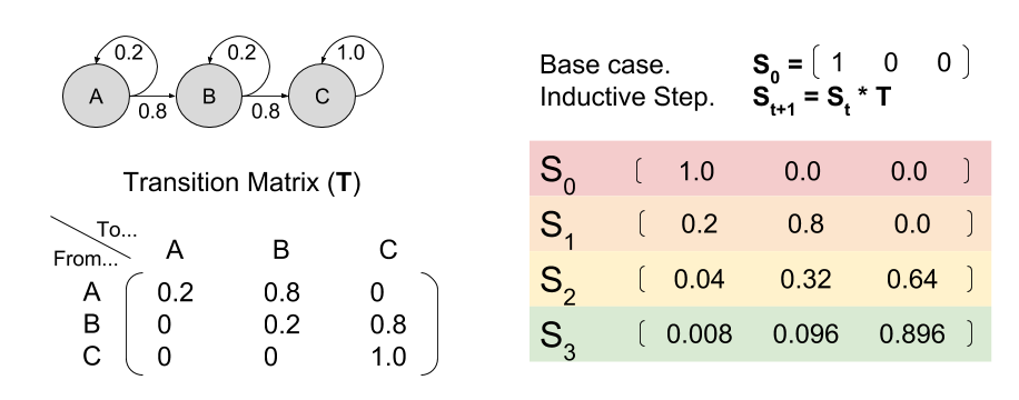
Extending Markov Chains
Recall that a Markov Chain contains a set of states S, and a transition model P. A Markov Decision Process (MDP) extends this device, by adding three new elements.
Specifically, an MDP is a 5-tuple (S, P, A, R, ɣ):
A set of states s ∈ S
A transition model Pa(s’ | s).
A set of actions a ∈ A
A reward function R(s, s’)
A discount factor ɣ
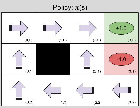
To illustrate, consider GridWorld. In this example, every location in this two-dimensional grid is a state, for example (1,0). State (3,0) is a desirable location: R(s(3,0)) = +1.0, but state (3,1) is undesirable, R(s(3,1)) = -1.0. All other states are neutral.
Gridworld supports four actions, or movements: up, down, left, and right. However, locomotion is imperfect: if Up is selected, the agent will only move up with 80% probability: 20% of the time it will go left or right instead. Finally, attempting to move into a forbidden square will simply return the agent to its original location (“hitting the wall”).
The core problem of MDPs is to find a policy (π), a function that specifies the agent’s response to all possible states. In general, policies should strive to maximize reward, e.g., something like this:
Why is the policy at (2,2) Left instead of Up? Because (2,1) is dangerous: despite selecting Up, there is a 10% chance that the agent will accidentally move Right, and be punished.
Let’s now consider an environment with only three states A, B, and C. First, notice how different policies change the resultant Markov Chain:
This observation is important. Policy determines the transition model.
Towards Policy Valuation V(s)
An agent seeks to maximize reward. But what does that mean, exactly?
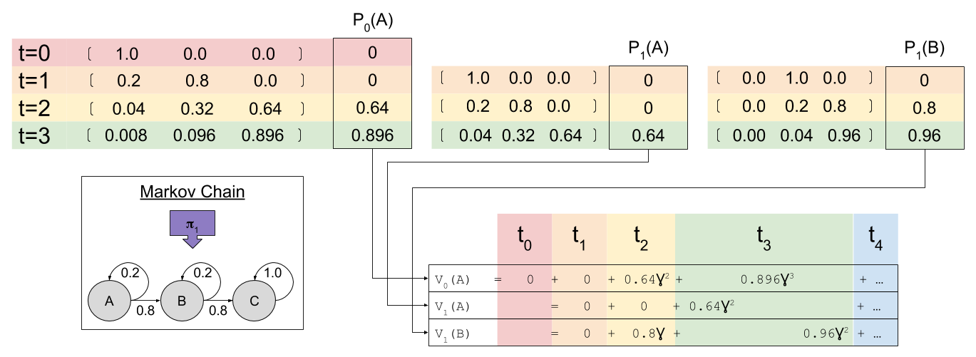
Imagine an agent selects 𝝅1. Given the resultant Markov Chain, we already know how to use matrix multiplication to predict future locations St. The predicted reward Pt is simply the dot product of expected location and the reward function.
We might be tempted to define the value function V(S) as the sum of all predicted future rewards:
However, this approach is flawed. Animals value temporal proximity: all else equal, we prefer to obtain rewards quickly. This is temporal discounting: as rewards are further removed from the present, their value is discounted.
In reinforcement learning, we implement temporal discounting with the gamma parameter: rewards that are k timesteps away are multiplied by the exponential discount factor . The value function becomes:
In our example, at time zero our agent starts in state A. We have already used linear algebra to compute our Pk predictions. To calculate value, we simply compute $latex \sum{\gamma^k P_k}$
Agents compute V(s) at every time step. At t=1, two valuations are relevant:
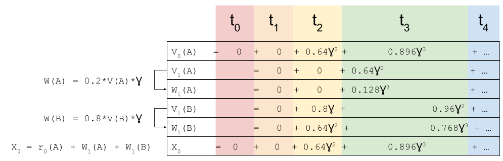
What is the relationship between the value functions at t=0 and t=1? To answer this, we need to multiply each term by , where is the state being considered at the next time step.
Similarly,
Critically, consider the sum :
Does look familiar? That’s because it equals ! In this way, we have a way of equating a valuation at t=0 and t=1. This property is known as intertemporal consistency.
Bellman Equation
We have seen that . Let’s flesh out this equation, and generalize to time t.
This is the Bellman Equation, and it is a central fixture in control systems. At its heart, we define value in terms of both immediate reward and future predicted value. We thereby break up a complex problem into small subproblems, a key optimization technique that can be approached with dynamic programming.
Next time, we will explore how reinforcement learning uses the Bellman Equation to learn strategies with which to engage its environment (the optimal policy 𝝅). See you then!
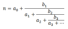
Have you run into simple continued fractions in your mathematical adventures? They look like this:
Let represent the coefficients and . If you fix you can uniquely represent with . For example:
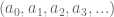
Let us call the leading coefficients of n. Here we have represented the rational with four coefficients. It turns out that every rational number can be expressed with a finite number of leading coefficients.
Irrational Numbers
Life gets interesting when you look at the leading coefficients of irrational numbers. Consider the following:
First note that these irrational numbers have an infinite number of leading coefficients.
What do you notice about ? It repeats, of course! What is the repeating sequence for ? The sequence .
How about ? Well, after the first two digits, we notice an interesting pattern then then . The value of this triplet is non-periodic, but easy enough to compute. The situation looks even more bleak when you consider the …
Thus (golden ratio) and feature repeating coefficients, but and (Euler’s number) do not. What differentiates these groups?
Of these numbers, only the transcendental numbers fail to exhibit a period. Can this pattern be generalized? Probably. 🙂 There exists an unproved conjecture in number theory, that all infinite, non-periodic leading coefficients with bounded terms are transcendental.
Real Approximation As Coefficient Trimming
Stare the digits of . Can you come up with a fraction that approximates it?
Perhaps you have picked up the trick that is surprisingly close:
But could you come up with from first principles? More to the point, could you construct a fraction that comes yet closer to ‘s position on the number line?
Decomposing these numbers into continued fractions should betray the answer:
We can approximate any irrational number by truncating . Want a more accurate approximation of ? Keep more digits:
I’ll note in passing that this style of approximation resembles how algorithms approximate the frequency of signals by discarding smaller eigenvalues.
About π
Much ink has been spilled on the number . For example, does it contain roughly equal frequencies of 3s and 7s? When you generalize this question to any base (not just base 10), the question becomes whether is a normalnumber. Most mathematicians suspect the answer is Yes, but this remains pure conjecture to-date.
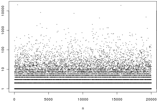
Let’s return to the digits of . Here is a graph of the first two hundred:
Do you see a pattern? I don’t.
Let’s zoom out. This encyclopedia displays the first 20,000 coefficients of :
So affords no obvious pattern. Is there another way to generate the digits of such that a pattern emerges?
Let quadratic continued fraction represent a number expressed as:
Set . Here only is allowed to vary. Astonishingly, the following fact is true:
Thus, continued fractions allow us to make sense out of important transcendental numbers like .
I’ll close with a quote:
Continued fractions are, in some ways, more “mathematically natural” representations of a real number than other representations such as decimal representations.
You remember algebra, and how annoying it was to use symbols that merely represented numbers? Statisticians get their jollies by terrorizing people with a similar toy, the random variable. The set of all possible values for a given variable is known as its domain.
Let’s define a discrete random variable called Happy. We are now in a position to evaluate expressions like Probability(Happy=true)
The domain of Happy is of size two (it can resolve to either true, or false). Since domain size is pivotal in this post, we will abbreviate it. Let an VariableN be a discrete random variable whose domain is size N (in the literature, the probability distribution for VariableN is known as the categorical distribution).
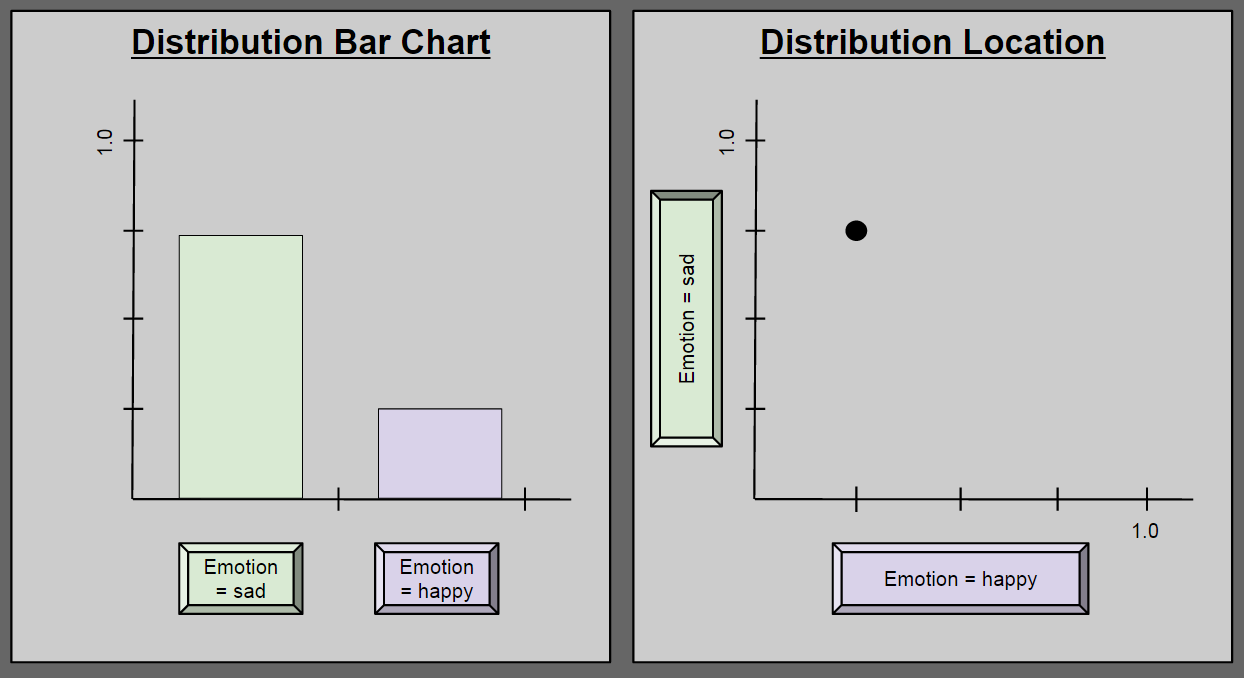
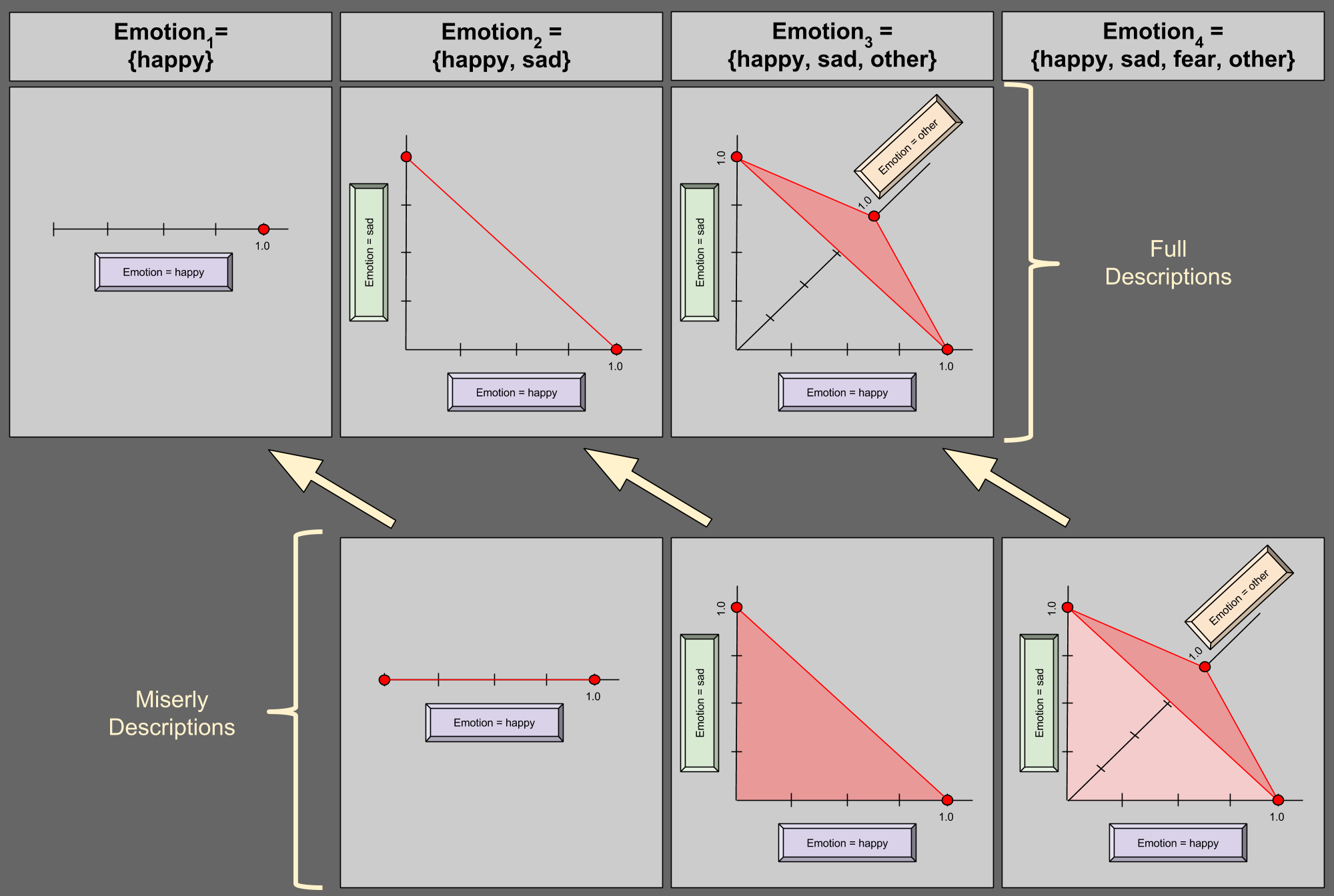
Consider a new variable, Emotion2 = { happy, sad }. Suppose we use this variable to describe a person undergoing a major depression. At any one time, such a person may have a 25% chance of being happy, and a 75% chance of being sad. This state of affairs can be described in two ways:
Pause here until you can explain to yourself why these diagrams are equivalent.
A Modest Explanation Of All Emotion
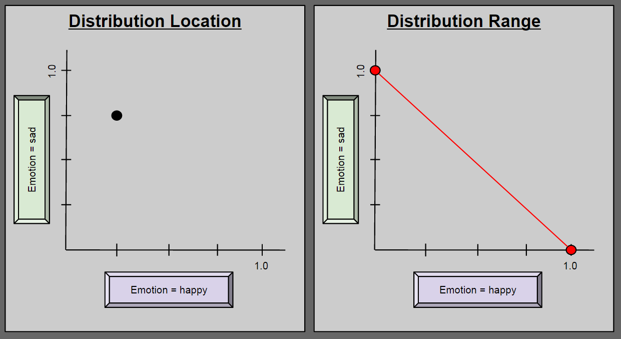
We have seen how a particular configuration of Emotion2 can accurately characterize a depressed person. But Emotion2 is intended to describe all possible human emotion. Can it take on any value in this two-dimensional space? No: to describe a human being as P(happy) = 1.5; P(sad) = -0.1 is nonsensical. So what values besides (0.25, 0.75) are possible for Emotion2?
The above range diagram (right side) answers our question: any instance of Emotion2 must reside along the red line. Take a second to convince yourself of this. It sometimes helps to think about the endpoints (0.0, 1.0) and (1.0, 0.0).
Bar Charts Are Hyperlocations
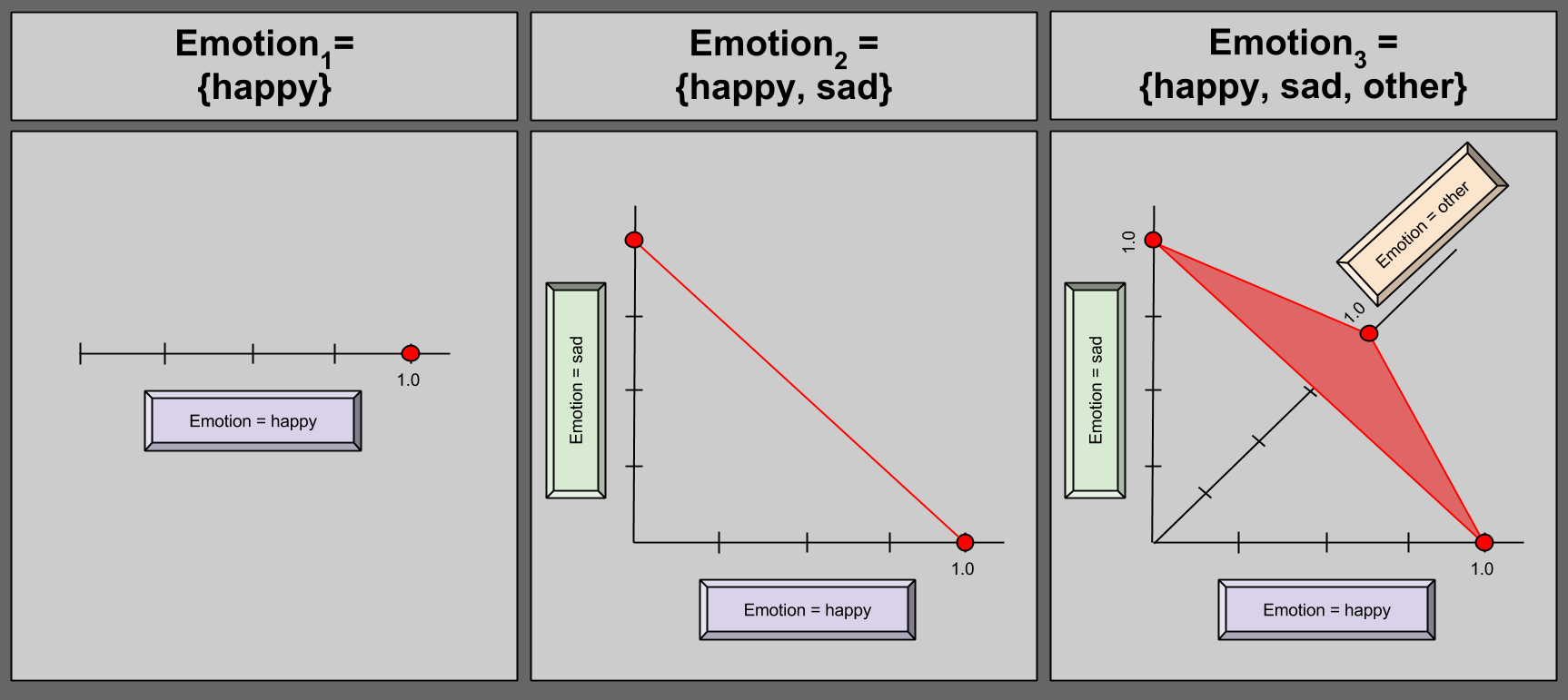
Perhaps you are not enthralled with the descriptive power of Emotion2. Perhaps you subscribe to the heresy that certain human experiences cannot be usefully described as either happy or sad. Let us expand our model to catch these “corner cases”, and define Emotion3 = { happy, sad, other }.
Can we identify a distribution range of this new variable? Of course!
Take a moment to convince yourself that Emotion3 may never contain any point outside the shaded red area.
Alright, so we have a fairly pleasing geometric picture of a discrete random variables with domains up to size 3. But what happens when we mature our model again? Imagine expanding our random variable to encapsulate the six universal emotions.
Could you draw a bar chart for an arbitrary Emotion6?
Of course you could; you’d simply need to add four more bars to the first diagram of this post.
Now, what about location in space?
Drawing in 6-D is hard. 🙂
Here is the paradox: a simple bar chart corresponds with a cognitively intractable point in 6-dimensional space. I hope you never look at bar charts the same way!
An aside that, despite the constant three being sloppily hardcoded into our mental software, it turns out that reasoning about hyperlocations – points in N-dimensional space – is an important conceptual tool. If I ever get around to summarizing Drescher’s Good and Real, you’ll see hyperlocations used to establish an intuitive guide to quantum mechanics!
Miserly Description
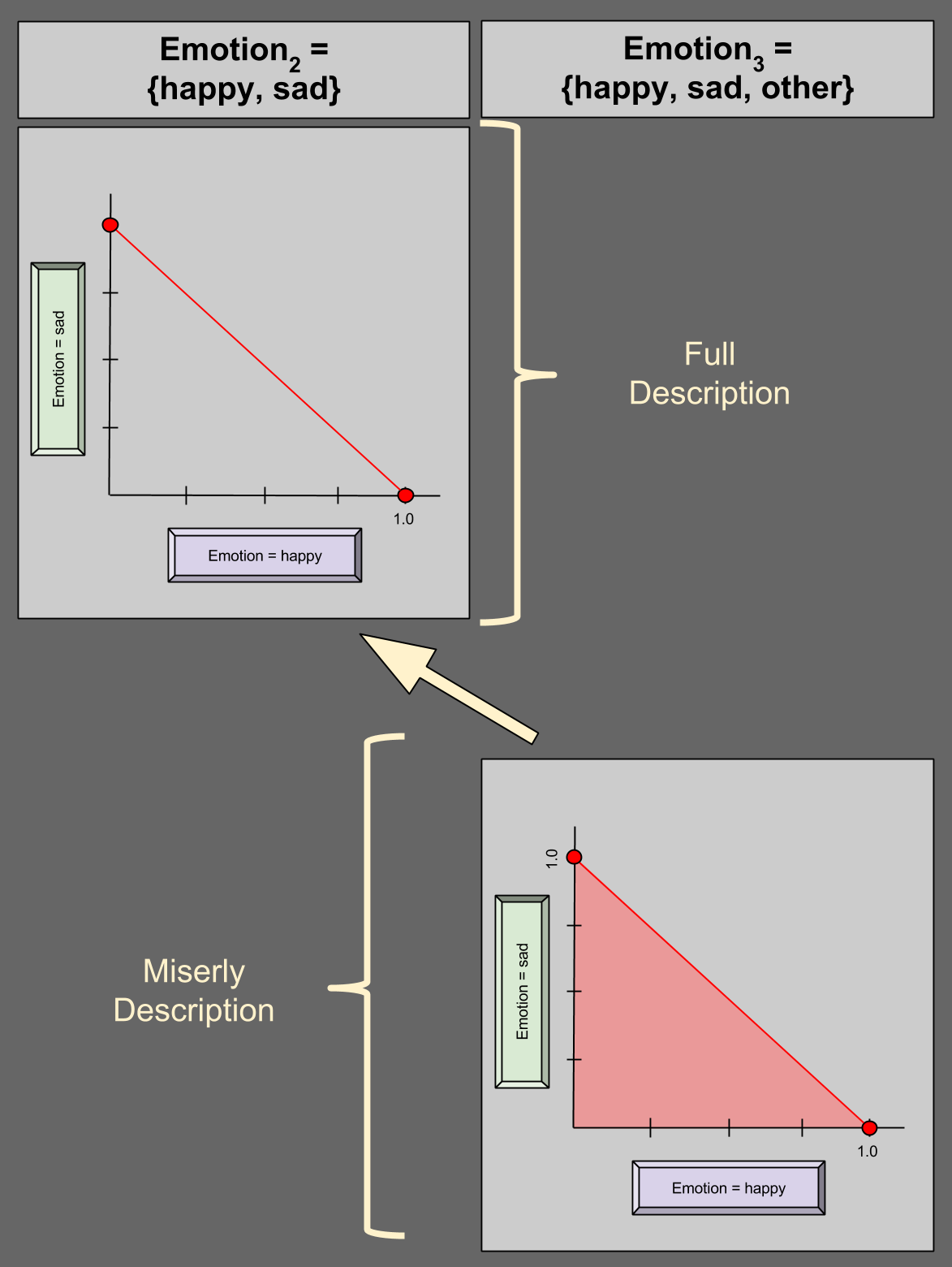
But do we really need 6-dimensional space to describe a domain of size 6? Perhaps surprisingly, we do not. Consider the case of Emotion3 = {happy, sad, other} again. Suppose I give you P(happy) = 0.5; P(sad) = 0.2. Do you really need me to tell you the P(other) = 0.3?
You could figure this out on your own, because the remaining 30% has to come from somewhere (0.3 = 1.0 – 0.5 – 0.2).
Given this fact that a variable has a 100% chance of being something (aka unitarity), we can describe a 4-variable in 3 dimensions:
In the bottom-right of the diagram, we see an illustration of miserly description. Suppose we are given (0.25, 0.25) for happy and sad, respectively. P(other) must then be valued at 0.5, and (0.25, 0.25) is thus a valid distribution – this is confirmed by its residence in the shaded region above. Suppose I give you any point on the dark red edge of the region (e.g., (1.0, 0.0)); what value for P(other) must you expect? Zero.
This generalizes: unitarity allows us to describe an N-variable in N-1 dimensions. Here are two more examples:
Notice the geometric similarities between the two descriptive styles, denoted by the yellow arrows.
The Hypervolume Of Probability
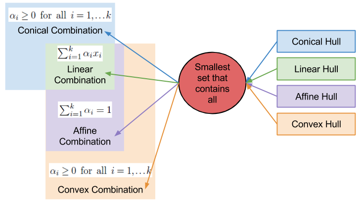
Consider the bottom row of our last figure (miserly descriptions). These geometric objects look similar: a triangle is not very different from a tetrahedron. What happens when we again move into a higher-dimensional space? Well, it turns out that there’s a name for this shape: a simplex is a generalization of a triangle into arbitrary dimensions. Personally, I would have preferred the term “hyperpyramid”, but I suppose the book of history is shut on this topic. 😛
We have thus arrived at an important result. The probability distribution associated with a discrete random variable can be represented as a simplex.
A Link To Convexity
I want you to recall my discussion on convex combinations.


 that can assume discrete values
  . Our partial understanding of the processes which determine
  . We would like to find some
  , which measures the uncertainty of this distribution.
 by combining events x2 and x3.

 and
and  . The uncertainty of two distributions is the sum of each individual uncertainty. Thus we add H(⅔, ⅓). But this distribution is reached only ½ of the time, so we multiply by 0.5.
 ? Consider a new
  , by definition.
  . Then we have:
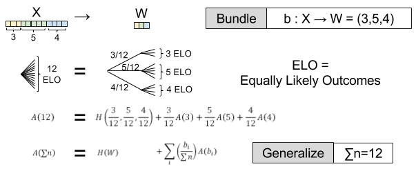
 . This simplifies things:
 does
does  hold? There is only one solution, as shown in Shannon’s paper:
 varies with logarithmic base (bits, trits, nats, etc). With this solution we can derive a general formula for entropy
  .
.

 )
) ← Found by arbitrary bundling (eg.,
  )
)
![K \left[ \sum{p_i \log(\sum{n_i})} - \sum{p_i \log(n_i)} \right]](https://s0.wp.com/latex.php?latex=K+%5Cleft%5B+%5Csum%7Bp_i+%5Clog%28%5Csum%7Bn_i%7D%29%7D+-+%5Csum%7Bp_i+%5Clog%28n_i%29%7D+%5Cright%5D&bg=ffffff&fg=555555&s=0&c=20201002)


 either
  or
or  or
or 
 if
if  then
then 
 then
then  s.t.
s.t.  iff
iff 
 over
over  , mixing both with the same third lottery
  in the same proportion α must not reverse that preference—adding identical “padding” is irrelevant to the choice.


 concavity to explain risk aversion? Prospect theory takes this approach yet further, and seeks to explain all of the above behaviors using a more complex shape
 represent our updated notion of utility. We can define expected prospect
  of a function as probability multiplied by the value function

 :
:
 , captures the status quo. Thus, the reference point allows us to differentiate gains and losses, thereby producing the endowment effect.

 has the following shape:
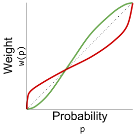


 , where


 :
:
 look familiar? That’s because it equals
  ! In this way, we have a way of equating a valuation at t=0 and t=1. This property is known as intertemporal consistency.
 . Let’
 and
and  . If you fix
  you can uniquely represent
  with
with 

 with four coefficients. It turns out that every rational number can be expressed with a finite number of leading coefficients.


 ? It repeats, of course! What is the repeating sequence for
  ? The sequence
  .
. ? Well, after the first two digits, we notice an interesting pattern
  then
then  then
then  . The value of this triplet is non-periodic, but easy enough to compute. The situation looks even more bleak when you consider the
  …
… (golden ratio) and
  feature repeating coefficients, but
  and
and  (Euler’s number) do not. What differentiates these groups?
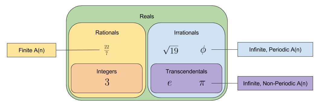
 is surprisingly close:


 . Here is a graph of the first two hundred:

 . Here only