Semirings As Algorithmic Parameters

Part Of: Graphical Models and Algebra sequence

In this, my final project in EE512A, I discuss how abstract algebra can be applied fruitfully in inference problems.

This project leverages some of the research conducted in the following posts:

My four page writeup is available here. My summary video is available here:

The Semiring Lifting Trick

Part Of: [Advanced Inference In Graphical Models] sequence

Table Of Contents

  • Motivations
  • Nested First-Order Semirings
  • Recursive Operator Resolution
  • Future Directions
  • Conclusion

Motivations

In 2002, Jason Eisner published Parameter Estimation for Probabilistic Finite-State Transducers in which he announced the discovery of the expectation semiring. This algebraic template is effectively used in the context of inferring parameters in a finite-state transducer (FST) model in the light of training data. The expectation semiring has the following structure:

Eisner- First-Order Semiring

Why are expectation semirings cool?

The weights from the expectation semiring are used to compute first-order statistics (e.g., the expected hypothesis length, or feature counts).

In 2009, Zhifei Li and Jason Eisner jointsly published First- and Second-Order Expectation Semirings with Applications to Minimum-Risk Training on Translation Forests.  This paper extended the previous paper by moving from a FST model to a hypergraph model, but also presented the variance semiring

Eisner- Second-Order Semiring

Why are variance semirings cool?

The variance semiring computes second-order statistics (e.g., the variance of the hypothesis length or the gradient of entropy). The variance semiring is thus essential for many interesting training paradigms such as minimum risk, deterministic annealing, active learning, and semi-supervised learning.

Our question today:

Is there a connection between these semirings?

Nested First-Order Semirings

To create a nested first-order ring, simply duplicate the original, and concatenate the two semirings together:

Eisner- Lifting Trick Part One

Notice the remapping section, where we map each nested pair to a single argument to the semiring operators. This is also captured in my use of color.

Recursive Operator Resolution

Once you have these re-mapped the nested semiring, you must simply apply the original operators repeatedly. It is worth noting that the original semiring interpreted ⊗ in terms of multiplication, so we must recast multiplication back to ⊗ as many times as we recurse into the operator chain.

Eisner- Lifting Trick Part Two (2)

As you can see, after our algebra machine finishes, the second-order semiring is synonymous with our previously-discovered result of the variance semiring.

Future Directions

So we possess a mechanism by which we can transform the expectation semiring into the variance semiring. Here’s a “before & after”:

Eisner- Lifting Trick Summary (1)

So what? Is this all just a post-hoc rationalization, an attempt to explain why the variance semiring is useful after the fact?

I believe not. Eisner is not the only theoretician using semirings, but he is the only one (to my knowledge) to propose second-order semirings.

How might other researchers go about discovering new second-order semirings? Well, one immediate first step would be to apply the lifting technique to known-viable semirings, and see what happens! 🙂

Conclusion

Let me conclude with my list of open questions:

  • Do any viable semirings known today in fact support the lifting trick?
  • Quarternions were derived from complex numbers, from (a+bi) to [(a+bi)+(c+di)j]. What explains this analogue?
  • Could third-order semirings be productive?

Injection, Surjection, Bijection

Part Of: Algebra sequence
Content Summary: 600 words, 6 min read

Function As Operator

A function can be conceived as a machine that converts input into output. For example:

Bijection- Function As Operator

Something cool noticed by geometers of long ago:

If I feed the above function ALL POSSIBLE NUMBERS, I get a line!

Function As Map

We can also view functions as maps, taking an input value & returning its corresponding output item.

Let domain represent the set of all numbers that an input could be. Let codomain represent the set of all numbers that an output could be.  For example:

bijection-function-as-map-1

Counting Edges

How might we classify different functions? One obvious thing to do is to count the number of edges entering or leaving a node:

bijection-counting-codomain-popularity

The definition of function is such that every input element maps to one and only one output element.  (This is why vertical lines are difficult to achieve in geometry). So the domain counts are relatively predictable.

The codomain numbers, on the other hand, are fairly interesting. We can distinguish popular outputs as those with more than one entry, and unpopular outputs as those with no entries.

Injection & Surjection (& Bijection)

Suppose we want a way to refer to function maps that produce no popular outputs, whose codomain elements have at most one element. Call such functions injective functions.

Suppose we want a way to refer to function maps with no unpopular outputs, whose codomain elements have at least one element. Call such functions surjective functions.

If neither popular nor unpopular outputs exist — if all outputs are “normal” 🙂 — we may call such functions bijective functions.

The above example is neither injective nor surjective:

bijection-all-three-properties

Examples of all four outcomes:

bijection-all-four-outcomes

Cardinality vs. Bijection

Consider the bottom-left example. Note that its domain is smaller than its codomain (3 < 4). If I let you rearrange the arrows any which way, could you manufacture surjection? Take a minute to convince yourself that you cannot. Do you see why there will always be at least one unpopular output? Consider the top-right example. Note that its domain is larger than its codomain (4 > 3). If I allow you to rearrange the arrows any which way, could you manufacture injection?

Take a minute to convince yourself that you cannot. Do you see why there will always be at least one popular output?

The argument you must use to convince yourself of the above is an analogue to the pigeonhole principle.

More generally, we find that:

Bijection- Domain Cardinality Implications (1)

You can also use the above properties to “work backwards”: for example, if two sets provide at least one bijection, their relative sizes (cardinalities) must be equal.

Generalizing To Morphisms

When in doubt, zoom out! Time to fall in love with category theory. 🙂

Functions that are grounded in set theory. But other types of structure-preserving maps have been studied:

Bijection- Generalizing Functions (1)

Injection/Surjection/Bijection were named in the context of functions. Wouldn’t it be nice to have names any morphism that satisfies such properties? Well, you’re in luck!

Bijection- Extending To Homomorphism (2)

Recall that bijection (isomorphism) isn’t itself a unique property; rather, it is the union of the other two properties.

It turns out that another interesting property to read out of maps is endomorphism: a map of an algebraic structure to itself. That makes three interesting properties. Let us explore how the sets of homomorphisms (a homomorphism is an general instance of a morphism, kind of like the instantiation of an abstract class in computer science) relate to each other:

Bijection- Set Relations Including Endomorphism

Decoding the above figure:

  • Hom set of homomorphisms
  • End → set of endomorphisms
  • Mon set of monomorphisms (i.e., injective morphisms)
  • Epi → set of epimorphisms (i.e., surjective morphisms)
  • Iso → set of isomorphisms (i.e., bijective morphisms)
  • Aut → set of automorphisms (i.e., bijective morphisms that also satisfy the endomorphic property)
  • →  contain only homomorphisms from some infinite structures to themselves.

Goodman: Semiring Parsing

Part Of: [Advanced Inference In Graphical Models] sequence

Table Of Contents

  • Introduction
  • Article Metadata
  • Item-Based Description
  • Candidate Semirings
  • Mechanizing Algorithm Construction
  • Algorithm-Metaring Diplomacy
  • Conclusion

Introduction

There are 1,024 logical permutations of rings/fields. Why is so much of the algorithmic research on them focused on one particular class of algebraic structure: the semiring? Why not the ring, or the pseudoring?

One answer can be made by appealing to historical accident. Semiring-based algorithm generation methods were championed most prominently by the Natural Language Processing (NLP) community, because the Chomsky–Schützenberger theorem unearthed deep connections between context-free grammars and certain noncommutative semiring algebras.

This post is a summary of John Goodman’s article, Semiring Parsing, which applies group theoretic techniques to already-known algorithms used by NLP researchers.

Article Metadata

  • Article: Semiring Parsing
  • Author: John Goodman
  • Published: 1999
  • Citations: 126 (note: as of 11/2014)
  • Link: Here (note: not a permalink)

Item-Based Description

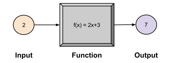
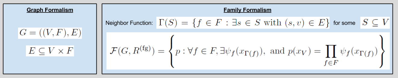
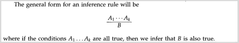
One major innovation in Goodman’s paper is item based descriptions. The syntax is straightforward:

Goodman- Item Syntax

This kind of notation simplifies the specification of parsers. More generally, as we will see, it will also free us from the traditional procedural-based approach to constructing algorithms in this domain.
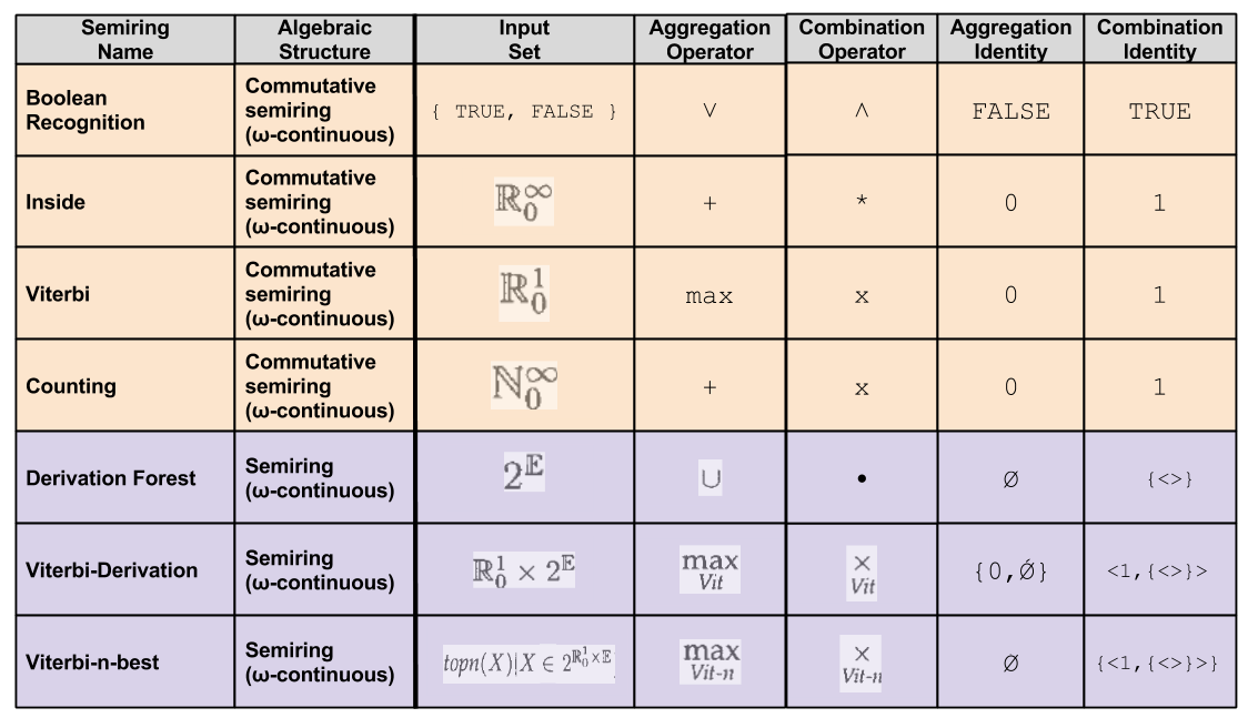
Semiring Types

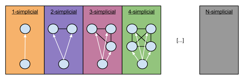
Let me call any type of permutation within a group-like structure a metagroup, and let me call any type of permutation within a ring-/field- like structure a metaring.

Another bit of background: do you remember the space of metarings? Here’s a diagram to refresh your memory:

Group Theory- Trimming Fields

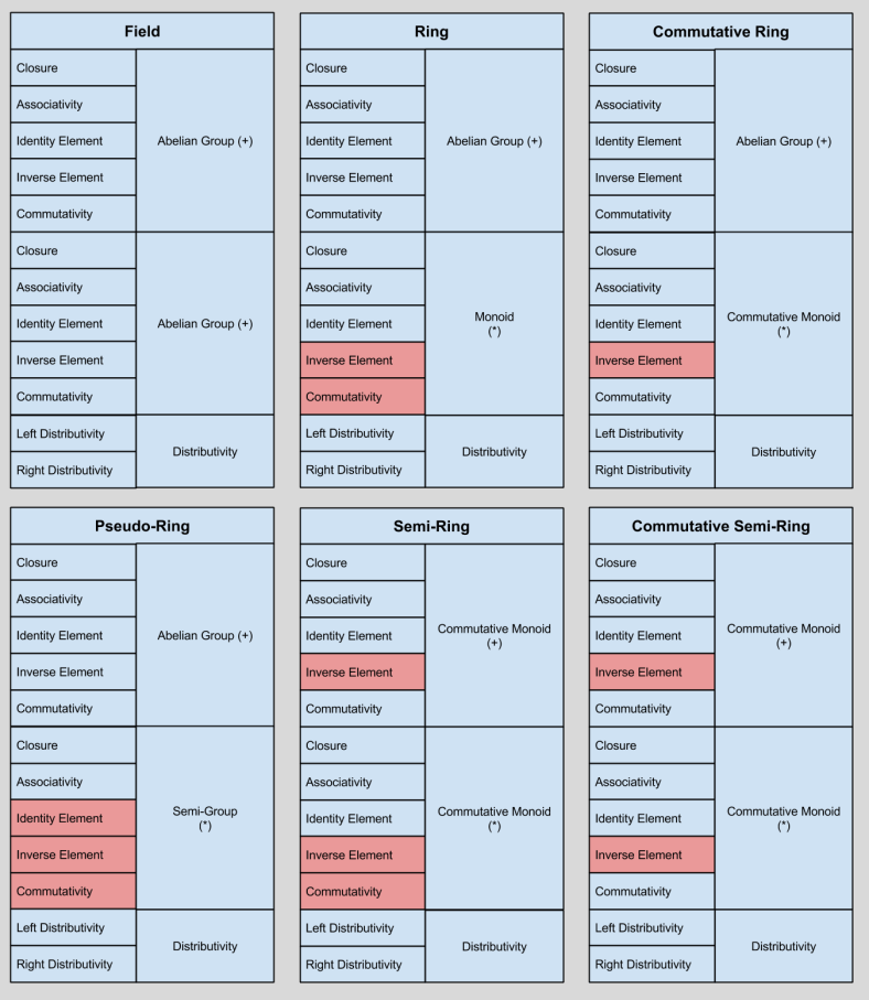
Ring-like algebraic structures only have five differentiating factors: the input set over which they operator, the aggregation operator, the combination operator, and their two identity elements.

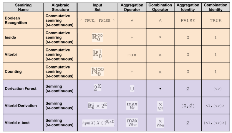
We can imagine a multitude of different permutations of these five variables. In the NLP community, seven permutations stand out as particularly valuable. They are:

Goodman- Semiring Types (3)

Mechanizing Algorithm Construction

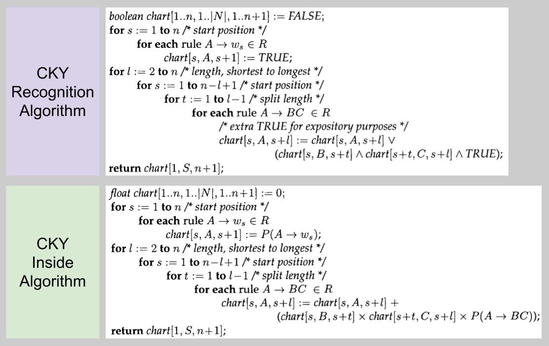
Consider the following algorithms:

Goodman- CKY recognition versus inside algorithm

Notice any similarities?

You should! The only differences between the two algorithms are substitutions between:

  • ˄ <–> *
  • ˅ <–> +
  • P(*) <–> TRUE

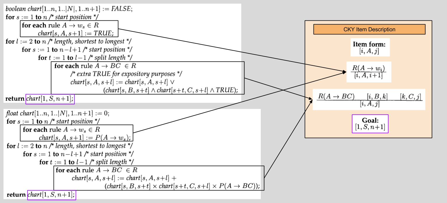
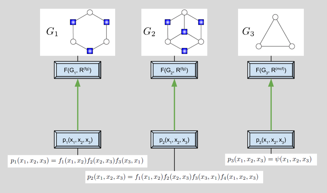
Let’s leverage item descriptions to generalize these two algorithms:

Goodman- Generalizing To Item-Based Description

With our new Item Description, algorithm generation becomes mechanized:

Goodman- Item-Based Description + Algebraic Structure = Algorithm

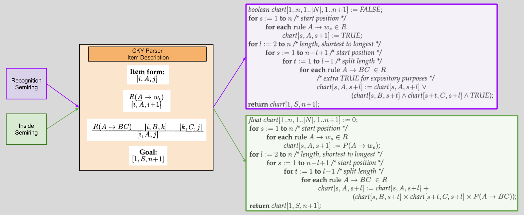
What makes this plug-and-play system more compelling than merely an ad-hoc explanation of algorithms whose existence we have already described?

Well, the Item Description doesn’t just accept these two semirings! Plug more in, and see what you get. 🙂 As Goodman puts it:

It [now becomes] easier to generalize parsers across tasks: a single item-based description can be used to compute values for a variety of applications, simply by changing semirings.

Algorithm – Metaring Diplomacy

Algorithms are often designed so that they can accept particular algebraic structures.

In typical practical Viterbi parsers, when two derivations have the same value, one of the derivations is arbitrarily chosen. In practice, this is usually a fine solution… but from a theoretical viewpoint, the arbitrary choice destroys the associative property of the additive operator, max. To preserve associativity, we keep derivation forests of all elements that tie for best.

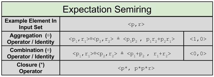
Computing over infinite sets is one powerful reason why commutivity is a desideratum for these metarings:

For parsers with loops, i.e., those in which an item can be used to derive itself, we will also require that sums of an infinite number of elements be well defined. In particular, we will require that the semirings be complete. This means that sums of an infinite number of elements should be associative and commutative, just like finite sums, and that multiplication should distribute over infinite sums, just as it does over finite ones.

Commutativity is shed in the three derivation-based semirings, for the simple reason that its multiplicative operator is designed to be order-preserving:

These semirings, unlike the other semirings described in Figure 5, are not commutative under their multiplicative operator, concatenation.

Swapping out semirings is not the only strategy to exploring parser diversity. One can also swap out the sets within the Item Descriptions.

Notice that each of the derivation semirings can also be used to create transducers. That is, we simply associate strings rather than grammar rules with each rule value. Instead of grammar rule concatenation, we perform string concatenation. The derivation semiring then corresponds to nondeterministic tranductions; the Viterbi semiring corresponds to a probabilistic transducer; and the Viterbi-n-best semiring could be used to get n-best lists from probabilistic transducers.

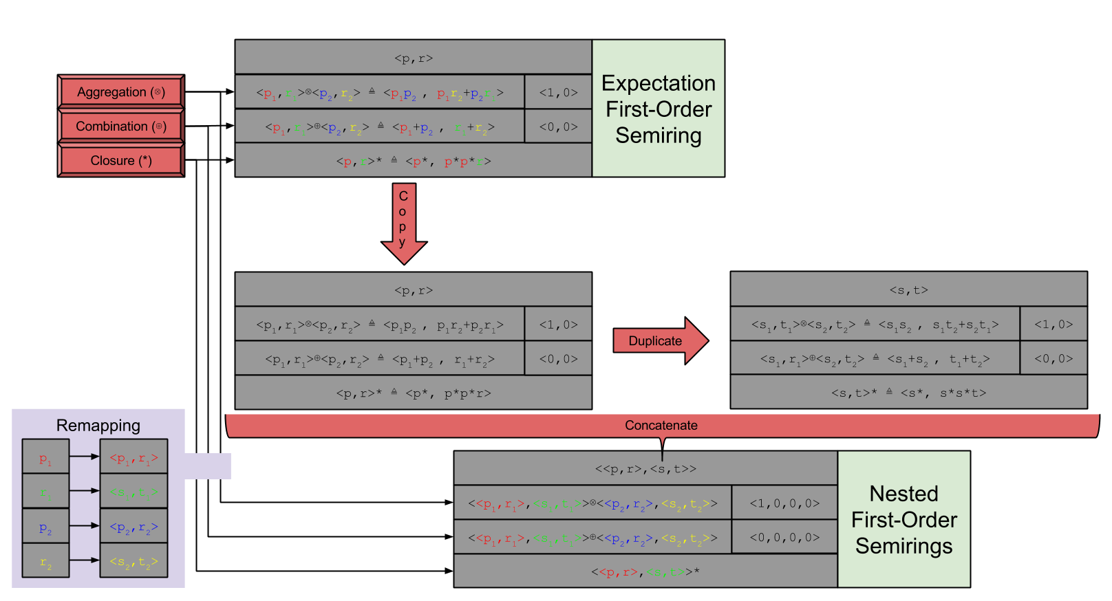
Think only two operators are allowed in a metaring? Think again!

Notice that [in the above example] we have multiplied an element of the semiring, V(D), by an integer, C(D, x). This multiplication is meantto indicate repeated addition, using the additive operator of the semiring. Thus, for instance, in the Viterbi semiring (max-product), “multiplying” (repeat-“addition”) by a count other than 0 has no effect, since x “+” x = max(x, x) = x. Whereas in the inside semiring (sum-product), repeat-“addition” corresponds to actual multiplication.

An interesting connection between finite-state automata and HMMs:

Nondeterministic finite-state automata (NFAs) and HMMs turn out to be examples of the same underlying formalism, whose values are simply computed in different semirings. Other semirings lead to other interesting values… For NFAs, we can use the boolean semiring to determine whether a string is in the language of an NFA; we can use the counting semiring to determine how many state sequences there are in the NFA for a given string; and we can use the derivation forest semiring to get a compact representation of all state sequences in an NFA for an input string. A single item-based description can be used to find all of these values.

Goodman in his paper calls for an extension of item-based descriptions:

It would be interesting to try to extend item-based descriptions to capture some of the formalisms ocvered by Koller, McAllester, and Pfeffer, including Bayes’ nets.

Conclusion

My Open Questions:

  • Have item-based descriptions since been extended? Is there active research on this front?

Concluding Quote:

In summary, the techniques of this paper will make it

  1. easier to compute outside values,
  2. easier to construct parsers that work for any ω-continuous semiring, and
  3. easier to compute infinite sums in those semirings.

In 1973, Teitelbaum wrote:

“We have pointed out the relevance of the theory of algebraic power series in noncommuting variables in order to minimize further piecemeal rediscovery”

We hope that this paper will bring about Teitelbaum’s wish.

An Introduction To Newcomb’s Paradox

Part Of: Algorithmic Game Theory sequence
Related To: An Introduction To Prisoner’s Dilemma
Content Summary: 1000 words, 10 min read

The Paradox

Newcomb’s Paradox is a thought experiment popularized by philosophy superstar Robert Nozick in 1969, with important implications for decision theory:

A superintelligence from another galaxy, whom we shall call Omega, comes to Earth and sets about playing a strange little game. In this game, Omega selects a human being, sets down two boxes in front of them, and flies away.

Box A is transparent and contains a thousand dollars.

Box B is opaque, and contains either a million dollars, or nothing.

You can take both boxes, or take only box B.

And the twist is that Omega has put a million dollars in box B iff Omega has predicted that you will take only box B.

Omega has been correct on each of 100 observed occasions so far – everyone who took both boxes has found box B empty and received only a thousand dollars; everyone who took only box B has found B containing a million dollars. (We assume that box A vanishes in a puff of smoke if you take only box B; no one else can take box A afterward.)

Before you make your choice, Omega has flown off and moved on to its next game. Box B is already empty or already full.

Omega drops two boxes on the ground in front of you and flies off.

Do you take both boxes, or only box B?

Well, what’s your answer? 🙂 Seriously, make up your mind before proceeding. Do you take one box, or two?

Robert Nozick once remarked that:

To almost everyone it is perfectly clear and obvious what should be done. The difficulty is that people seem to divide almost evenly on the problem, with large numbers thinking that the opposing half is just being silly.

The disagreement seems to stem from the contradiction of two strong intuitions: one “altruistic” intuition in favor of 1-box, the other 2-box intuition is more “selfish”. They are, respectively:

  1. Expectation Intuition: Take the action with the greater expected outcome.
  2. Maximization Intuition: Take the action which, given the current state of the world, guarantees you a better outcome than any other action.

Allow me to visualize the mechanics of this thought experiment now (note that the Predictor is a not-necessarily-omniscient version of Omega):

Newcomb's Paradox- Setup

Still with me? 🙂 Good. Let’s see if we can use game theory to mature our view of this paradox.

Game-Theoretic Lenses

Do you remember Introduction To Prisoner’s Dilemma? At one point in that article, we decomposed the problem into a decision matrix. We can do the same thing for this paradox, too:

Newcomb's Paradox- Decision Matrix

From the perspective of the Decider, strategic dominance here cash out our Intuition #1: the bottom row always outperforms the top row.

However, the point of making the Predictor knowledgeable is that landing in the gray cells (top-right, bottom-left) become unlikely. Let us make the size of our boxes represent the chance that they will occur.

Newcomb's Paradox- Predictive Accuracy Weighting

With a Predictor of infinite accuracy,  the size of the gray cells becomes zero, and now 1-Boxing suddenly dominates 2-Boxing.

With a Predictor with bounded intelligence, what follows? Might some logic be constructed to describe optimal choices in such a scenario?

A Philosophical Aside

Taken from this excellent article:

The standard philosophical conversation runs thusly:

  • One-boxer: “I take only box B, of course. I’d rather have a million than a thousand.”
  • Two-boxer: “Omega has already left. Either box B is already full or already empty. If box B is already empty, then taking both boxes nets me $1000, taking only box B nets me $0. If box B is already full, then taking both boxes nets $1,001,000, taking only box B nets $1,000,000. In either case I do better by taking both boxes, and worse by leaving a thousand dollars on the table – so I will be rational, and take both boxes.”
  • One-boxer: “If you’re so rational, why ain’cha rich?”
  • Two-boxer: “It’s not my fault Omega chooses to reward only people with irrational dispositions, but it’s already too late for me to do anything about that.”
  • One-boxer: “What if the reward within box B are something you could not leave behind? Would you still fall on your sword?”

Who wins, according to the experts? No consensus exists. Some relevant results, taken from a survey of professional philosophers:

Newcomb’s problem: one box or two boxes?

Accept or lean toward: two boxes 292 / 931 (31.4%)
Accept or lean toward: one box 198 / 931 (21.3%)
Don’t know 441 / 931 (47.4%)

Prediction Is Time Travel

There is a wonderfully recursive nature to Newcomb’s problem: the accuracy of the predictor stems from it modelling your decision machinery.

Newcomb's Paradox- Decision Process Leakage

In this (more complete) diagram, we have the Predictor building a model of your cognitive faculties via the proxy of behavior.

As the fidelity of its model (gray image in the Predictor) improves as more information is pulled from the Decider (red arrow) the more perfect its predictive accuracy, (reduced size of the gray outcome-rectangles).

The Decider may say to herself:

Oh, if only my mind were such that the “altruistic” Expectation Intuition could win at prediction-time, but the “selfish” Maximization Intuition could win at choice-time.

Then, I would deceive the Predictor. Then, I would win $1,001,000.

But even if she possesses the ability to control her mind in this way, a perfect Predictor will learn of it. Thus, the Decider may reason:

If my changing my mind is so predictable, perhaps I might find some vehicle to change my mind based on the results of coin-flip…

What the Decider is trying to do, here, is a mechanism to corrupt the Predictor’s knowledge. How might a Predictor respond to such attacks of deterministic prediction?

Open Questions

This article represents more of an exploration, than a tour of hardened results.

Maybe I’ll produce revision #2 at some point… anyways, to my present self, the following are open questions:

  • How can we get clear on the relations between Newcomb’s Paradox and game theory more generally?
  • How might the “probability mass” lens be used to generalize this paradox to non-perfect Predictors
  • How might the metaphysics of retroactive causality, or at least the intuitions behind such constructs, play into the decision?
  • How much explanatory power does the anti-maximization principle behind 1-boxing (and the ability to precommit to such “altruistic irrationality”) say about human feelings of guilt or gratitude?
  • How might this subject be enriched by complexity theory, and metamathetics?
  • How might this subject enrich discussions of reciprical altruism and hyperbolic discounting?

Until next time.

Tree, Generalized

Part Of: [Advanced Inference In Graphical Models] sequence
Followup To: [An Inference Trail To Chordal Graphs]

Table Of Contents

  • Context
  • Parallels Between Trees and Chordal Graphs
  • Parameterizing Simpliciality
  • Definition By Construction
  • K-trees
  • Takeaways

Parallels Between Trees And Chordal Graphs

In Murderous Messages, we defined perfect elimination orderings as follows:

Let perfect elimination ordering (PEO) refer to exact inference algorithms that do not at any step introduce fill-in edges; F = {}. In order to accomplish such an ordering, we should eliminate nodes that match either one of two elimination principles:

  • have only zero or one neighbor (leaf nodes)
  • have neighbors that are already fully connected. (simplicial nodes)

In our inference trails towards both trees and chordal graphs, we came upon the following similar-looking properties:

  • Every tree with size > 1 has two leaf nodes (nodes in a tree with only one neighbor).
  • A chordal graph is either a clique, or at least two non-adjacent nodes are simplicial. [Lemma 30]

Note the implication that you’ll never run out of leaf/simplicial nodes to eliminate: every time you remove a leaf/simplicial node, the resultant tree/graph still retains this two-target characteristic. Since you are assured leaves/simplicials “all the way down”, this guarantees that both trees and chordal graphs may sustain perfect elimination orders. And that is nice.

We proceeded to author construction-based definitions of these data structures. Note again how frustratingly similar they are, despite their independent derivations!

  • T is a tree if it is generated via the following process: Start with a node v. Repeatedly choose a next vertex, and connect it with an edge to exactly one previously chosen vertex.
  • G is a chordal graph if generated via the following process: Start with a clique. All chordal graphs can be generated by connecting the next node to some set of previously-chosen nodes that are a clique. [Corollary 36]

Parameterizing Simpliciality

Let’s transcend an appeal to coincidence: why have two things when we can have one? 😛

Time to consolidate. Recall our definition of simplicial node?

Simplicial node: a node whose neighbors form a clique.

Let’s make this definition more granular, and define a concept that hinges on the size of this neighbor-clique.

k-simplicial node: a node whose neighbors form a clique of size k.

Here’s how this looks “in action”:

EE512 Generalizing Trees- N-simplicials

A few notes about the boundaries of this distribution:

  • What is the maximum size of an k-simplicial node? When the entire graph is a clique, when k = N (the number of all nodes). k spans [1..N].
  • Does a 1-simplicial node remind you of anything? It should. Creating a 1-simplicial node is equivalent to appending a leaf node.

Definition By Construction

With this definition of k-simplicials in hand, let’s return to our twin construction properties mentioned above.

  • T is a tree if generated via the following process: Start with a node v. Repeatedly choose a next vertex, and connect it with an edge to exactly one previously chosen vertex.
  • G is a chordal graph if generated via the following process: Start with a clique. All chordal graphs can be generated by connecting the next node to some set of previously-chosen nodes that are a clique. [Corollary 36]

Now, we can represent this graphically by realizing that the former process is about consistently appending 1-simplicials, and the latter process fueled by k-simplicials. The distinction, then, looks like this:


EE512 Generalizing Trees- Tree Construction Basics (1)

k-Trees

In our visualization of tree construction, did you notice how the color of tree construction doesn’t change? Let’s generalize this property beyond orange (1-simplicials).

Let k-tree represent a tree whose construction process is fueled by k-simplicials. I illustrate four of these tree abstractions here:

EE512 Generalizing Trees- k-Trees

Are there k-trees that are not chordal graphs? How do k-trees generally relate to our previous concepts of trees and chordal graphs? Another illustration should clarify these inter-relationships:

EE512 Generalizing Trees- Tree Hierarchy

A tree is a subset of a k-tree which is a subset of chordal graphs. We know this because:

  • A chordal graph is constructed by (any chain of) simplicials
  • A k-tree is constructed by (one consistent chain of) simplicials.
  • A tree is constructed by (one particular consistent chain of) simplicials.

Takeaways

  • A leaf node is synonymous with a simplicial node of size 1.
  • A k-tree is a tree constructed with simplicial nodes of size k (a 1-tree is synonymous with a tree, per the above identity).
  • A tree is a kind of k-tree which is a kind of chordal graph: these three data structures are strict subsets of one another.

Here’s a consolidation of the above images, for convenience:

EE512 Generalized Trees- Summary Infographic (1)

Designer Families

Part Of: [Advanced Inference In Graphical Models] sequence
Followup To: [Family vs. Universe]

Table Of Contents

  • Motivations
  • Graph Type: Factor Graphs
  • Graph Type: Markov Random Fields
  • A Tale Of Three Families
  • On Specificity
  • Takeaways

Motivations

Today, we’re going to talk through the construction of a family, and how such a construction might succeed or fail.

Across machine learning, there exist dozens of different graph types; of these, three are the most popular:

  1. Markov Random Fields
  2. Factor Graphs
  3. Bayesian Networks

Our example today will span the first two of these graphs.

Graph Type: Markov Random Field

Markov Random Fields (MRFs) have very simple semantics; they are basically undirected graphs:

EE512 Designer Families- MRF Example


In the above MRF, we have a graph with five vertices and six edges. It’s probability distribution is comprised of three factors, one per maximal clique (the first term corresponds to top-left triangle, etc).

The graphical model of MRFs can be formalized by defining its graph and rule structure. Let us define the following terms:

  • Let V represent the set of all vertices in the graph
  • Let E represent the set of all edges in the graph

We now define the Markov Random Field:

EE512 Designer Families- MRF Theory

Here’s how I “translate” all the math on the right:

  • “For each cliques in the set of all maximal cliques, there exists a function phi over some collection of variables within the clique.”
  • “The joint probability, then, over all variables is the product of all  phi functions in the graph.”

It turns out that there are several other rules which describe an MRF equally well, but maximal-clique factorization rule serves our purposes here well enough.

Introducing Factor Graphs

Factor graphs (FGs) also have undirected edges, but they honor other constraints, as well:

EE512 Designer Families- Factor Graphs Example

Notice anything interesting about this graph’s edges? […] Did you notice how no v-nodes or f-nodes are never connected one another? In other words, if we group all edges Graphs with this property, that all edges span across two distinct nodesets, are called bipartite graphs.

How is the probability distribution formula constructed? […] On inspection, it becomes clear that each of the four terms on the right-hand side correspond to factor-nodes.

A rigorous definition of factor graphs simply require us to generalize these two observations. First, some vocabulary is in order.

  • Let V represents the set of vertex-nodes on the graph (e.g., v1 through v3)
  • Let F represent the set of factor-nodes on the graph (e.g., f1 through f4)
  • Let E represent the set of all edges in the graph.

We are now in a position to completely specify the Factor Graph:

EE512 Designer Families- Factor Graphs Theory

Here’s how I would translate this family definition:

  • “Let neighbor function RHO be defined as a function that searches through each factor and returns each neighbor.”
  • “For every factor f, there exists a function PSI, which takes as its input all neighbors of f (those neighbors discovered by RHO).”
  • “The joint probability is then the product of all such functions PSI.”

 A Tale Of Three Families

Ready to get your hands dirty?! Good! Let’s consider three specific graphs: two factor graphs, and one Markov Random Field:

EE512 Designer Families- Three Families

Does this diagram make sense? If not, let me explain each family-distribution pairing in turn.

  • The leftmost family represents the semantics of factor-graphs R(fg), along with a set of factor-nodes, vertex-nodes, and edges G1. Just as in the factor-graph example above, its corresponding probability distribution is derived from these two elements: each term corresponding to one factor-node and its neighbors.
  • The center family is identical to the previous factor-graph, except for an additional factor-node. This additional element corresponds to an extra term in the resultant probability distribution, f4(…)
  • The rightmost family represents the semantics of MRFs (here, maxclique factorization) R(mcf), along with a set of nodes and edges G3. Its probability distribution flows from the semantics: since all three variables form a clique, the distribution is a factor across all variables.

So far, so obvious. But recall the purpose of rules: they deliver yes/no answers to any probability distribution that applies for membership. Thus, we must be willing in inquire whether p1 is a member of Family2, etc.

Here are the membership results of the six new family applications:

EE512 Designer Families- Three Families With Exclusions


A green edge (A, B) means that our Ath distribution is a member of our Bth family. In contrast, a red edge denotes non-membershipLet me explain the results of each new edge in turn:

  1. (1,2) is green because f(a, b) -> g(x, y, z) transforms are possible.
  2. (1,3) is green because f(a, b) -> g(x, y, z) transforms are possible.
  3. (2,1) is red because f(a, b, c) -> g(x, y) transforms are impossible (if they were, they would be expressed as two-term factors originally).
  4. (2,3) is green because f(a, b, c) -> g(x, y, z) transforms are possible.
  5. (3,1) is red because f(a, b, c) -> g(x, y) transforms are impossible (similar reasoning to (2,1)).
  6. (3,2) is green because f(a, b, c) -> g(x, y, z) transforms are possible.

On Specificity & Generality

Consider you find yourself asked to design an graphical model that includes p1 within its family. As you can see, any of the above graphs satisfy this requirement. But that does not make them equal.

When designing families, we ought to be as narrow as possible. Suppose we don’t particularly care to compute over p2 or p3. Then, we have reason to prefer Familyasdf – it has the power to say No to these irrelevant distributions, and thereby save computational resources.

Here’s how my professor summarizes & illustrates this principle:

This suggests that there are two aspects of a type of graphical model that indicate its power, and that is: generality, can a graph be found such that its family includes a given distribution; and specificity, how discriminative is a given graph that represents a given distribution.

For example, a collection of all i.i.d. random variables would trivially be a member of all of the aforementioned families, but such a distribution would violate many of the properties that are left unspecied. We might be interested in another graphical model semantics that specifically precludes those cases.

These two notions help us get clear on the kinds of questions to ask when designing a graphical model from scratch.

Takeaways

  • When designing a family, one must optimize not just for generality (admitting viable distributions). Specificity (the rejection of irrelevant distributions) matters just as much.

Murderous Messages

Part Of: [Advanced Inference In Graphical Models] sequence
Followup To: [Murderous Cliques]

Table Of Contents

  • Context
  • Forests & Trees
  • Perfect Elimination
  • Murderous Messages
  • Takeaways

Context

Our takeaways from last time:

  • Cliques are graph subsets that are fully connected.
  • Variable elimination is a computational process that first bundles like factors together, and then eliminates a variable via “summing it out”.
  • The order in which one eliminates irrelevant variables is computationally significant.
  • Sometimes, variable elimination creates undesirable fill-in edges – edges that breach the family contract & expands the boundaries of the graphical model.
  • Fill-in edges happen because the former neighbors of a fill-in edge must form a clique.
  • In conclusion, when selecting the order in which to eliminate variables, if possible, choose the variable whose neighbors already form a clique.

We can make our conclusion more specific.

Let perfect elimination ordering refer to exact inference algorithms that do not at any step introduce fill-in edges; F = {}.

In order to accomplish such an ordering, we should eliminate nodes that match either one of two elimination principles:

  1. have only zero or one neighbor
  2. have neighbors that are already fully connected.

In either case, fill-in edges will not be added because the clique requirement is already satisfied.

Forests & Trees

So far in this sequence, we have considered a wide variety of different graph types. Today, let us consider a special type of graph: the forest, and the tree.

Informally, a forest is a graph that has no cycles. A tree is a connected forest, a forest in which two nodes are connected by precisely one path.

Below is one forest comprising four trees:

EE512 Messages- Tree Illustration


Theorem 2 (Trees, Berge). Let T = (V, E) be an undirected graph with |V| = n > 2. Then each of the following properties are equivalent and each can be used to define a tree.

  1. G is connected, and has no cycles.
  2. G has n – 1 edges and has no cycles.
  3. G is connected and contains exactly n-1 edges.
  4. G has no cycles, and if an edge is added to G, exactly one cycle is created.
  5. G is connected, and if any edge is removed, the remaining graph is not connected.
  6. Every pair of vertices of G is connected by one unique path.
  7. G can be generated via the following process: Start with a node v. Repeatedly choose a next vertex, and connect it with an edge to exactly one previously chosen vertex.

Perfect Elimination

Do all graphs support a perfect elimination ordering (PEO)? Consider the following:

EE512 Messages- PEO Examples

In the left image, a PEO does not exist: it doesn’t matter which node you chose, its two neighbors are not already-connected. The right image, in contrast, does contain a PEO (as was shown last time).

Notice how the left 4-cycle is not a tree, whereas the right chain is. Might other types of trees (besides chains) also support perfect elimination orderings? The answer turns out to be yes:

  • The maximum clique size of a tree is 2 (cliques of size three would form a cycle, and trees do not contain cycles).
  • Every tree with size > 1 has 2 leaf nodes (nodes in a tree with only one neighbor).
  • Variable elimination on trees do not destroy their tree-like nature.
  • If you always choose to eliminate an edge node first, the neighboring clique is of size 1, which guarantees F = {}. Let us call this procedure leaf-first ordering.
  • Locating leaf nodes on a tree is computationally straightforward.

Therefore, any leaf-first ordering on a tree will yield a perfect elimination order, and operate in O(N*r^2) time.

Two important facts to remember:

  1. The leaf-first ordering procedure does not specify one particular ordering as correct. Rather, it denotes a group of orderings as equivalent and correct.
  2. As a data structure, trees were chosen because they guarantee elimination principle #1.

Murderous Messages

Time to view leaf-first ordering in action. Consider a tree T with |V| = 15. Suppose that, after building this tree with statistical data, a scientist submits a query as to the relationship between two variables.

We know how to perform this inference: eliminate all variables not involved in the query itself. To perform such elimination perfectly, we perform leaf-first ordering:

EE512 Messages- Murderous Messages

In the right image, we “rooted” T on the query variables, and eliminated the irrelevant nodes starting from the “lowest” ones.

Pay attention to the way information flows with the above ordering. It is as if the query variables act as a collecting magnet, sucking information from the rest of the graph towards its nodes. On a Bayesian interpretation of this algorithm, we can meaningfully state that this leaf-first ordering is a collection of evidence. Let us call such transmission of evidence message passing.

We can then re-interpret leaf-first ordering in the following protocol:

Message Passing Protocol (MPP): A message may be sent from node i to a neighbor node j only after node i has received a message from all of its other neighbors.

We motivated the MPP based on trees, and elimination principle #1. But we will later MPP in the context of chordal graphs, which guarantee principle #2.

Two things to bear in mind as we close:

  • The phrase murderous messages is simply a playful concatenation of the more cantankerous “variable elimination message passing”.
  • Notice how the requirement for maximal efficiency (in the form of perfect elimination ordering) is what motivated us to connect an inference algorithm with notions of epistemic fidelity.

Takeaways

  • A forest is a graph that has no cycles. A tree is a connected forest.
  • In trees, perfect elimination ordering is accomplished by leaf-first ordering.
  • Leaf-first ordering can be reasonably interpreted as the collection of evidence (a.k.a message passing, or belief propagation).