An Introduction To Bayesian Inference

bayes

Motivations

Bayesianism is a big deal. Here’s what the Stanford Encyclopedia had to say about it:

In the past decade, Bayesian confirmation theory has firmly established itself as the dominant view on confirmation; currently one cannot very well discuss a confirmation-theoretic issue without making clear whether, and if so why, one’s position on that issue deviates from standard Bayesian thinking.

What’s more, Bayesianism is everywhere:

In this post, I’ll introduce you to how it works in practice.

Probability Space

Humans are funny things. Even though we can’t produce randomness, we can understand it. We can even attempt to summarize that understanding, in 300 words or less. Ready? Go!

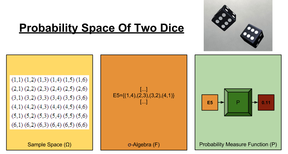
A probability space has three components:

  1. Sample Space: A set of all possible outcomes, that could possibly occur. (Think: the ingredients)
  2. σ-Algebra. A set of events, each of which contain at least one outcome. (Think: the menu)
  3. Probability Measure Function. A set of probabilities, which convert events into numbers ranging from 0% to 100% (Think: the chef).

To illustrate, let’s carve out the probability space of two fair dice:
Bayes- Probability Space of Two Dice (1)

You remember algebra, and how annoying it was to use symbols that merely represented numbers? Statisticians get their jollies by terrorizing people with a similar toy, the random variable. The set of all possible values for a given variable is its domain.

Let’s define a discrete random variable called Happy.  We are now in a position to evaluate expressions like:

P(Happy=true)

Such an explicit notation will get tedious quickly. Please remember the following abbreviations:

P(Happy=true) \rightarrow P(happy)

P(Happy=false) \rightarrow P(\neg{happy})

Okay, so let’s say we define the probability function that maps each manifestation of Happy’s domain to a number. What about when you take other information into account? Is your P(happy) going to be unaffected by learning, say, the outcome of the 2016 US Presidential Election? Not likely, and we’d like a tool to express this contextual knowledge. In statistics jargon, we would like to condition on this information. This information will be put on the RHS of the probability function, after a new symbol: |

Suppose I define a new variable, ElectionOutcome = { republican, democrat, green } Now, I can finally make intelligible statements about:

P(happy | ElectionOutcome=green)

A helpful subvocalization of the above:

The probability of happiness GIVEN THAT the Green Party won the election.

Bayescraft

When I told you about conditioning, were you outraged that I didn’t mention outcome trees? No? Then go watch this (5min). I’ll wait.

Now you understand why outcome trees are useful. Here, then, is the complete method to calculate joint probability (“what are the chances X and Y will occur?”):

Bayes- Conditional Probability

The above tree can be condensed into the following formula (where X and Y represent any value in these variables’ domain):

P(X, Y) = P(X|Y)*P(Y)

Variable names are arbitrary, so we can just as easily write:

P(Y, X) = P(Y|X)*P(X)

But the joint operator (“and”) is commutative: P(X,Y) = P(Y,X). So we can glue the above equations together.

P(X, Y) = P(Y|X)*P(X)

Since both of the equations above are equal to P(X, Y), we can glue them together:

P(X|Y)*P(Y) = P(Y|X)*P(X)

Dividing both sides by P(Y) gives us Bayes Theorem:

P(X|Y) = \frac{P(Y|X) * P(X)}{P(Y)}

“Okay…”, you may be thinking, “Why should I care about this short, bland-looking equation?”

Look closer! Here, let me rename X and Y:

P(Hypothesis|Evidence) = \frac{P(Evidence|Hypothesis) * P(Hypothesis)}{P(Evidence)}

Let’s cast this back into English.

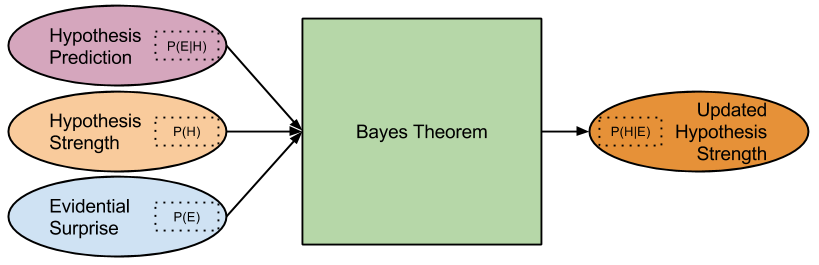
  • P(Hypothesis) answers the question: how likely is it that my hypothesis is true?
  • P(Hypothesis|Evidence) answers the question: how likely is my hypothesis, given this new evidence?
  • P(Evidence) answers the question: how likely is my evidence? It is a measure of surprise.
  • P(Evidence|Hypothesis) answers the question: if my hypothesis is true, how likely am I to see this evidence? It is a measure of prediction.

Shuffling around the above terms, we get:

P(Hypothesis|Evidence) = P(Hypothesis) * \frac{P(Evidence|Hypothesis)}{P(Evidence)}

We can see now that we are shifting, by some factor, from P(Hypothesis) to P(Hypothesis|Evidence). Our beginning hypothesis is now updated with new evidence. Here’s a graphical representation of this Bayesian updating:
Bayes- Updating Theory

DIY Inference

A Dream

Once upon a time, you are fast asleep. In your dream an angel appears, and presents you with a riddle:

“Back in the real world, right now, an email just arrived in your inbox. Is it spam?”

You smirk a little.

“This question bores me! You haven’t given me enough information!”
“Ye of little faith! Behold, I bequeath you information, for I have counted all emails in your inbox.”
“Revelation 1: For every 100 emails you receive, 78 are spam.”
“What is your opinion now? Is this new message spam?”
“Probably… sure. I think it’s spam.”

The angel glares at you, for reasons you do not understand.

“So, let me tell you more about this email. It contains the word ‘plans’.”
“… And how does that help me?”
“Revelation 2: The likelihood of ‘plans’ being in a spam message is 3%.”
“Revelation 3: The likelihood of it appearing in a normal message is 11%”
“Human! Has your opinion changed? Do you now think you have received the brainchild of some marketing intern?”

A fog of confusion and fear washes over you.

“… Can I phone a friend?”

You wake up. But you don’t stop thinking about your dream. What is the right way to answer?

Without any knowledge of its contents, we viewed the email as 78% likely to be spam. What changed? The word “plans” appears, and that word is more than three times as likely to occur in non-spam messages! Therefore, should we expect 78% to increase or decrease? Decrease, of course! But how much?

Math Goggles, Engage!

If you’ve solved a word problem once in your life, you know what comes next. Math!

Time to replace these squirmy words with pretty symbols! We shall build our house as follows:

  • Let “Spam” represent a random variable. Its domain is { true, false }.
  • Let “Plans” represent a random variable. Its domain is { true, false }

How might we cast the angel’s Revelations, and Query, to maths?

Word Soup Math Diamonds
“R1: For every 100 emails you receive, 78 are spam.” P(spam) = 0.78
“R2: The likelihood of ‘plans’ being in a spam message is 3%.” P(plans|spam) = 0.03
“R3: The likelihood of it appearing in a normal message is 11%” P(plans|¬spam) = 0.11
“Q: Is this message spam?” P(spam|plans) = ?

Solving The Riddle

Of course, it is not enough to state a problem rigorously. It must be solved. With Bayes Theorem, we find that:

P(spam|plans) = \frac{P(plans|spam)P(spam)}{P(plans)}

Do we know all of the terms on the right-hand side? No: we have not been given P(plans). How do we compute it? By a trick outside the scope of this post: marginalization. If we marginalize over Plans (i.e., sum over all instances of its domain), we spawn the ability able to compute P(E). In Mathese, we have:

P(spam|plans) = \frac{P(plans|spam)P(spam)}{P(plans,spam)+ P(plans,\neg{spam})}

P(plans,spam) and P(plans, ¬spam) represent joint probabilities that we can expand. Applying the Laws of Conditional Probability (given earlier), we have:

P(spam|plans) = \frac{P(plans|spam)P(spam)}{P(plans|spam)P(spam) + P(plans|\neg{spam})P(\neg{spam})}

Notice we know the values of all the above variables except P(¬spam). We can use an axiom of probability theory to find it:

Word Soup Math Diamonds
“Every variable had 100% chance of being something.” P(X) + P(¬X) = 1.0.

Since the P(spam) is 0.78, we can infer that P(¬spam) is 0.22.

Now the fun part – plug in the numbers!

P(spam|plans) = \frac{0.03 * 0.78}{(0.03*0.78) + (0.11*0.22)} = 0.49159

Take a deep breath. Stare at your result. Blink three times. Okay.

This new figure, 0.49, interacts with your previous intuitions in two ways.

  1. It corroborates them: “plans” is evidence against spam, and 0.49 is indeed smaller than 0.78.
  2. It sharpens them: we used to be unable to quantify how much the word “plans” would weaken our spam hypothesis.

The mathematical machinery we just walked through, then, accomplished the following:

Bayes- Updating Example

Technical Rationality

We are finally ready to sketch a rather technical theory of knowledge.

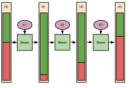
In the above example, learning occured precisely once: on receipt of new evidence. But in real life we collect evidence across time. The Bayes learning mechanism, then, looks something like this:
Bayes- Updating Over Time

Let’s apply this to reading people at a party. Let H represent the hypothesis that some person you just met, call him Sam, is an introvert.

Suppose that 48% of men are introverts. Such a number represents a good beginning degree-of-confidence in your hypothesis. Your H0, therefore, is 48%.

Next, a good Bayesian would go about collecting evidence for her hypothesis. Suppose, after 40 minutes of discretely observing Sam, we see him retreat to a corner of the room, and adopt a “thousand yard stare’. Call this evidence E1, and our updated introversion hypothesis (H1) increases dramatically, say to 92%.

Next, we go over and engage Sam in a long conversation about his background. We notice that, as the conversation progresses, Sam becomes more animated and personable, not less. This new evidence E2 “speaks against” E1, and our hypothesis regresses (H2 becomes 69%).

After these pleasantries, Sam appears to be more comfortable with you. He leans forward and discloses that he just got out of a fight with his wife, and is battling a major headache. He also mentions regretting being such a bore at this party. With these explanatory data now available, your introversion hypothesis wanes. Sure, Sam could be lying, but the likelihood of that happening, in such a context, is lower than truth-telling. Perhaps later we will encounter evidence that induces an update towards a (lying) introvert hypothesis. But given the information we currently possess, our H3 rests at 37%.

Wrapping Up

Resources

In this post, I’ve taken a largely symbolic approach to Bayes’ Theorem. Given the extraordinary influence of the result, many other teaching strategies are available. If you’d like to get more comfortable with the above, I would recommend the following:

Takeaways

I have, by now, installed a strange image in your head. You can perceive within yourself a sea of hypotheses, each with their own probability bar, adjusting with every new experience. Sure, you may miscalculate – your brain is made of meat, after all. But you have a sense now that there is a Right Way to do reason, a normative bar that maximizes inferential power.

Hold onto that image. Next time, we’ll cast this inferential technique to its own epistemology (theory of knowledge), and explore the implications.

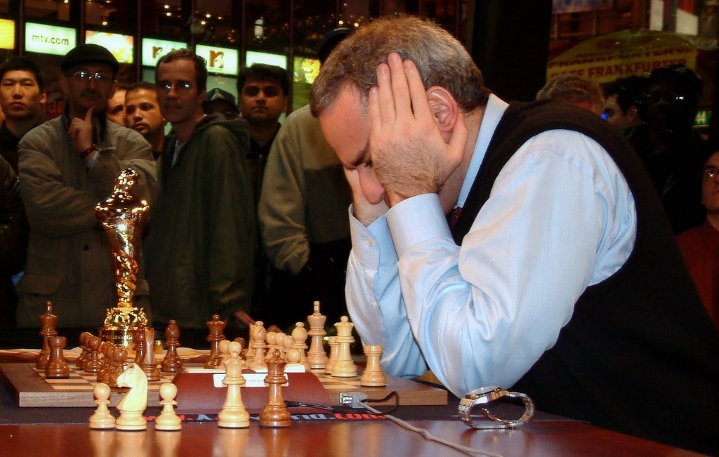
[Sequence] Decision Making In Chess

grandmaster_tournament

Designed for people who know little more than how the chess pieces move, this series introduces the game, and scans its results for lessons we can apply to how we understand life more generally.

  1. An Introduction To Chess.  Surveys chess culture and illustrates chess evaluation, bringing attention to the often-subconscious nature of the latter.
  2. Decision Trees In Chess. Explores how the decision trees and the minimax algorithm can capture the entirety of chess gameplay.
  3. The Chess SuperTree. Having exploring single-move decisions, this post zooms out to consider the game of chess as a whole – its complete game tree.
  4. The Psychology Of Chess. Compares these computer science & game theoretic approaches to chess with hints on how the brain uses somatic markers & heuristics to decide more efficiently.

An Introduction To Chess


kasparov

Content advisory: if you know how chess pieces move, this article should be accessible to you.

Table Of Contents

  • Introduction
    • Why Does This Article Exist?
    • Notation & Scoring
    • Ratings & Phases
    • How Chess Games Are Won
  • How To Understand A Chess Position
    • Introducing My Starting Position
    • Towards Board Analysis
    • Why Are Goals Important In Chess?
    • Finding A Goal
    • Anticipating The Other Player
    • How Does Chess Become Less Mysterious?
  • How To Evaluate A Chess Decision
    • Introducing My Solution
    • Analyzing Decision Outcome
    • Towards Judgment
  • Conclusion
    • Takeaways

Introduction

Why Does This Article Exist?

I have played chess professionally since I was a teenager. Today, I want to share with you this private world. I will use a correspondence game (multiple days per move, instead of seconds per move) to do this. We will together walk through several decisions made by myself and my opponent.

My reasons for exploring chess are not contained to sharing an interesting piece of my life. I hope to use this material to explore certain themes useful in attempts to integrate artificial intelligence and cognitive psychology. But that’s for later. For now, if you leave this article with a better idea of how chess players make decisions, I will be content.

In a former life, I taught chess to hundreds of six-year-olds. While clearly my readership here will need more guidance, I will do my best to accomodate. 😉

Notation & Scoring

The 64 squares of the chessboard have names. Rows (also called ranks) are 1-8, columns (also called files) are a-h.

square_names

Piece symbols are:

  • King: K
  • Queen: Q
  • Rook: R
  • Bishop: B
  • Knight: N
  • Pawn: [blank]

Algebraic notation allows us to communicate chess moves. To do this, we simply combine the two symbols discussed above. There exist a few caveats regarding captures (x means capture) and when more than one piece can land on a particular square (originating rank or file is appended). Examples:

  • Ne4 would represent a Knight that moved to the e4 square.
  • gxf5 would represent a pawn on g4 that captures something on the f5 square.
  • Rec8 would represent a Rook on e8 moving to c8, if another Rook could have moved to the same location.

Chess players like to keep track of how large their army is, compared to their opponent.  However, it is not enough to count pieces: a queen is certainly worth more than a pawn. The following scoring system was instead invented, to facilitate comparison between different combinations of pieces:

  • King: [infinite points]
  • Queen: 9 points
  • Rook: 5 points
  • Bishop: 3 points
  • Knight: 3 points
  • Pawn: 1 point

Ratings & Phases

The chess community tracks playing strength with a fairly complex rating scheme: ELO ratings. Absolute beginners tend to perform around a 400 rating, those who play regularly-yet-casually trend towards 900, and world champions hover around 2800. The relationship between effort and rating is non-linear: almost all chess players will tell you that more time is required to rise from 1900 to 2100, than from 1200 to 1900. (My rating is currently 1903.)

The game of chess is traditionally divided into three separate phases: the opening, the middlegame, and the endgame. Since all games start from the same position, chess players have gradually accumulated common wisdom in the form of opening lines. Professional chess players will often memorize the first 5-15 moves of nearly every possible (interesting) game: to fail to memorize these lines is to risk independently trying to reconstruct them, failing to compute the optimal sequence, and finding yourself at a disadvantage (for this reason, tournament preparation can be quite competitive, and taxing). Similarly, endgames typically feature very few pieces, its complexity becomes tractable, and memorization returns to the fore as an extremely important tool.

It is a very normal sight to see grandmaster chess players play their first opening moves quickly, consume hours lost in thought during the middlegame, and as soon the endgame result is clear either resign or offer a draw – the end result being nearly inevitable. Arguably, the middlegame retains the most interest in the face of such professionalism. Why? Because our best minds have failed to tame its complexities.

How Chess Games Are Won

Chess games are won by checkmate: i.e., attacking the enemy King in a way it cannot escape. But checkmating is not an unpredictable “happening”. After your tenth chess game or so, you will start to notice that the cumulative strength of one’s army is predictive of the final outcome. This is why the scoring system above was developed: to allow for the prediction of victory.

Most absolute beginners have little difficulty accepting the scoring system.  The next realization, however, takes significantly longer to arrive. You see, for most players in chess, material advantages come about by accident. An understanding of attack and defense, the eyesight needed to anticipate “tricks”: these take a long time to mature (such mistakes feel like dropping a negative sign in a long algebra problem).

It takes a long time for the average human to transcend mistake-avoidance in chess. If you keep at it, your idea of how material advantages come about will slowly evolve. The key moment comes when both players are mature enough to avoid material-shedding mistakes. Despite this newfound sophistication, you are not guaranteed to avoid losing material. Why? Well… every so often, your opponent will make a series of attacking threats, and you will find yourself simply unable to generate an adequate defense response. Here come the critical question: how can one player be able to outpace his opponent in this way?

The answer lies in positional advantages, a concept much more subtle than material advantages. There are very many ways for a player to possess a positional advantage. These positional features include:

  • Pawn structure. Some pawn configurations are more stable and defensible than others.
  • Space. Some pawn configurations allow a player relatively more room to maneuver.
  • King safety. How many defensive resources does a player have near his King?
  • Piece development. At what rate has one managed to bring pieces into the fight?
  • Piece cohesion. Are one’s pieces working together well?
  • Initiative. Who is making more threats, and dictating the course of the game?

The above discussion can, perhaps, be represented with the following (rather crude) diagram:

Chess Advantages

How To Understand A Chess Position

Introducing My Starting Position

With these preliminaries out of the way, I can now to introduce you to real gameplay!

Consider the following. Each player have played 19 moves, I am playing as White, and it is my turn.

posA

Towards Board Analysis

Taking what we learned about How Chess Games Are Won, let us now conduct a material analysis and a positional analysis.

Black and White possess an equal number of pawns, knights, bishops, rooks, queen. Materially, then, the game is even. This equality is likely to persist: White shouldn’t play Bxe7 because Black can recapture Rxe7, and Black comes out ahead 2 pts. Similarly, if Black were to capture Bxc3, this isn’t necessarily wrong, but after Qxc3 material remains even (both players have lost 3 pts).

But chess is not just about the size of your army, it is how the army is being used. Let us scan through our positional features using a -5 to 5 scale (-5 is a strong Black advantage, 5 is a strong White advantage, 0 is equality):

  • Pawn structure: +0.2. (Both sides pawn’s coordinate well, and are not particularly vulnerable to attack.)
  • Space. +2.0. (My pawns have advanced, on average, 1 or 2 steps further.)
  • King safety. -1.8. (My King doesn’t have a guardian Bishop, and my pawns are further advanced.)
  • Piece development. +0.2. (No pieces are “stuck at home” anymore.)
  • Piece cohesion. +0.8 (Black’s Bb7 and Rc8 aren’t particularly useful, White’s Rooks and Bishops are better coordinated.)
  • Initiative. +0.0 (Neither player has significant control over the pace of the game.)

I want to emphasize here that the above numbers are subjective: I made them up. But, as we shall see later, quantifying my “gut feelings” turns out to be extremely useful.

Let us also notice that most pieces, on both sides, are not attacking the pieces of the other player. There are simply too many pawns in the way. It turns out that, in clogged positions such as these, play tends toward aggressive pawn moves that serve to clear a path for one’s pieces. Such “jailbreaking” often happens after subtle maneuvering, where each player tries to get her pieces better positioned to capitalize on their coming freedom.

Why Are Goals Important In Chess?

Why should play tend to gravitate towards aggressive pawn moves? Consider what happens if one player contents himself with moving his pieces behind his wall of pawns. His opponent could then dictate when and where to bring the fight to the other player.

This kind of argument illustrates a central theme in chess: successful players tend to think in terms of goals. Once a goal is selected, a plan must then be constructed, to move the current situation towards the desired one. Let’s now turn to my starting position to see what this means, concretely.

Finding A Goal

White desires to find a goal from his current position. We’ve already agreed that aggressive pawn moves represent useful goals. But where?

Is White best advised to locate a Queenside strategy? Can White aggressively advance his a- or b- pawn on the Queenside? Not immediately: such moves (a5 and b4) would lose material. What if White were to, say, play Na2 – thus making possible a later b4 pawn advance (since both Queen and Knight can now recapture). This plan does not seem especially promising: after a future b4 cxb4, Black’s Queen and a Rook will suddenly be attacking our pawn on c4!

How about a Kingside strategy, with White advancing his g and/or h pawns? Too risky: White’s King is already rather exposed.  White’s biggest space advantage is in the center of the board, so let’s now restrict our attention there. The two candidates are: e5 and f5.

center_strategies

Can White afford to advance his pawn to e5 (left image)? Do the math! 20. e5 dxe5 21. fxe5 Nxe5 22. Rxe5 Bxe5. Black comes out way ahead (if you didn’t do the math, take my word for it :P).

So 20. e5 is no good. How 20. f5 (right image)? This is safe: gxf5 is met by exf5 – equality. But such a move allows Black’s Knight to land in the e5 square (Ne5), previously impossible when the f4 pawn could capture such a daring Knight. So, White seems in a quandary: he would like to increase his space advantage… but both pawn moves that could accomplish this seem deficient.

We know that White should be playing in the center. Perhaps White’s goal should be: arrange his pieces so that e5 does not lose material.

Anticipating The Other Player

What goals should Black try to pursue? Can we anticipate counterplay?

On the Queenside, b5 qualifies as a pawn break. For now, it loses material. Let us imagine a future position where it does not lose material. Is such a goal worthy of Black’s time? Perhaps: it will take a while to get his pieces ready, but it would give Black an attack.

On the Kingside, Black will hesitate to advance his pawns, due to safety concerns for his King.

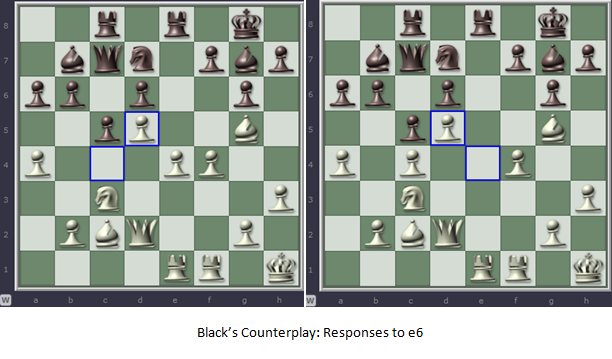
In the Center, f5 will ultimately weaken Black’s pawn structure. But what should happen if Black plays e6? White may hesitate to capture: dxe6 fxe6 gives up White’s space advantage. So, Black will have the opportunity to capture exd5, after which White will face a choice. The following image imagines this choice (after 20. Bc2 e6 21. Kh1 exd5):

center_counterplay

Recapturing cxd5 (left image) preserves his central dominance, but now White must fear a very powerful Queenside attack: Black may now play c4 and Nc5. This threat is sufficiently scary: White will probably recapture exd5 (right image).

This possibility adds some urgency to White’s plan: if Black is given opportunity to play e6, he will bring the game closer to equality by relieving spatial pressure by trading pawns and Rooks. Worse still, such a trade would prevent White from meeting his goal to play e5!

How Does Chess Become Less Mysterious?

Pause for a minute, and take stock of how you feel.  You probably feel lost, a bit like you’ve wandered into a foreign land.  It turns out that almost everyone encountering this material has a similar experience. But this feeling of confusion is important, so let’s try to understand it.

Perhaps the strangeness comes from unfamiliarity. Or, perhaps my arguments lack specificity! Would you become able to confidently teach this new understanding of chess to a friend, dear reader, if I had only made it more lengthy, more precise?

I doubt it. Such an “improvement” feels funny once you consider how chess is learned. Playing strength does not improve once playing strength by argumentation (conscious reasoning) alone: experience must play a role.  Let us name this observation, that language can express chess knowledge more easily than it can teach it, representational language asymmetry.

I have watched literally hundreds of games play out from this exact pawn structure, and I have developed a very sharp intuition for what kinds of strategies matter in this type of position. In this four-pawns-Benoni, of course White must not find a goal on the Queenside. Likewise, the solution I employ below seems shocking at first… but it is a highly stylized pattern that I have, again, evaluated in the context of dozens of other games.

I have noticed representational language asymmetry before, while teaching ESL last year.  In my view, learning chess is a lot like learning a language: personal practice and learning from the example of others is the most efficient way forward.

How To Evaluate A Chess Decision

Dear reader, where have we landed? We now know that White would like to break through in the center. We also know that White is in crisis: he would like to act before Black plays e6, but all available pawn breaks lose material. What should White do?

Rather than motivate how I addressed this challenge, let me simply show you. 🙂

Introducing My Solution

20. e5 dxe5
21. f5

posA123

Analyzing Position Outcome

Material analysis:

  • I have lost one pawn (but no more: 21 …gxf5 22. Rxf5 is simply a trade).

Positional analysis:

  • Pawn structure: -0.5 (Black’s e5 pawn is now unopposed by any White pawn, but the e7 pawn is no discouraged from moving)
  • Space. +3.5. (My pawn on f5 really cramps his style! )
  • King safety. +0.5. (My pawn on f5 is looking to remove one of Black’s King’s protective pawns)
  • Piece development. +0.0. (No real changes in this feature.)
  • Piece cohesion. +4.5 (My Rooks are now active, my Knight and Bishops are now well-positioned, his Bishop is now blocked).
  • Initiative. +2.0 (White has started to dictate which aspects of the game are worthy of attention.)

Towards Judgment

We can now directly compare before and after!  Copying the two sets of numbers I produced above:

Starting Score End Score Difference
Material: Points +0.0 -1.0 -1.0
Position: Pawn structure +0.0 -0.5 -0.5
Position: Space +2.0 +3.5 +1.5
Position: King safety -1.5 +0.5 +2.0
Position: Piece development +0.0 +0.0 +0.0
Position: Piece cohesion +1.0 +4.5 +3.5
Position: Initiative +0.0 +2.0 +2.0

We see that I have accepted losses in material and pawn structure, in exchange for gains in space, King safety, piece cohesion, and initiative. But how are we to know whether such a complex tradeoff is a decision worth making?

Recall our vocabulary words: positional advantage, material advantage. Now is the time to admit cumulative advantage into our corpus. If we wish to speak intelligibly about chess decisions, we simply must compress our analysis features into a single number (there is no room for incommensurability in chess!).  Here’s how I view the cumulative effect of my decision:

Starting Score End Score Difference
Estimated Total +0.4 +0.6 +0.2

Dear reader, how am I to convince you that such a total score is correct? Will I provide you with cute mathematics? A weighted average over the above features?

I cannot provide such a thing, because I do not possess it. The truth is, I don’t consciously use mathematical reasoning while playing chess! Rather, all of my valuations are written in the currency of intuitions, of emotional valence. And that is a deep and mysterious thing.

Conclusion

Takeaways

Congratulations! You survived to the end of this article. We have covered a lot of ground. 🙂

I’ll close by recapping the points I most want you to remember:

  • Positional advantages cause material advantages, which in turn lead to checkmate.
  • Positional advantages are composed of many different features, such as pawn structure or piece cohesion.
  • Goals are vital to success.
  • Evaluating a chess position is a largely subconscious experience, one that requires experience.

Enjoy the +100 bump in chess rating I just gave you! 😉

Nietzsche: God is Dead

Context

It is no secret that human beings are terrible about thinking about politics and religion.  Every in-group has its own collection of pet ideas (its own semiosphere). And every single one of these massive cultural apparati are apt to go awry:

  • Arguably, some pro-intellectual groups have gotten history wrong (c.f., the Galileo affair).
  • Arguably, some anti-intellectual groups have gotten biology wrong (c.f., natural selection).
  • Arguably, some anti-religion groups have gotten philosophy wrong (c.f., logical positivism).

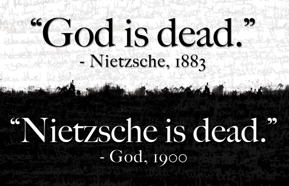
Today, I’d like to illustrate a “culture war” meme whose origins some pro-religion groups have gotten wrong: the phrase “God is dead”. I do this for three reasons:

  1. The meme is still misused frequently, yet its correction is less well-known than to the three other errors above.
  2. Nietzsche is an exceptionally interesting writer.
  3. To explain why I view the cognitive science of religion as a subject worthy of our attention.

Below I reproduce where “God is Dead” comes from: a parable.

From Nietzsche’s The Gay Science

The Madman

Have you not heard of that madman who lit a lantern in the bright morning hours, ran to the marketplace, and cried incessantly, “I seek God! I seek God!” As many of those who do not believe in God were standing around just then, he provoked much laughter. Why, did he get lost? said one. Did he lose his way like a child? said another. Or is he hiding? Is he afraid of us? Has he gone on a voyage? Thus they yelled and laughed. The madman jumped into their midst and pierced them with his glances.

“Whither is God” he cried. “I shall tell you. We have killed him – you and I. All of us are his murderers. But how have we done this? How were we able to drink up the sea? Who gave us the sponge to wipe away the entire horizon? What did we do when we unchained this earth from its sun? Whither is it moving now? Whither are we moving now? Away from all suns? Are we not plunging continually? Backward, sideward, forward, in all directions? Is there any up or down left? Are we not straying as through an infinite nothing? Do we not feel the breath of empty space? Has it not become colder? …

Do we not smell anything yet of God’s decomposition? Gods too decompose. God is dead. God remains dead. And we have killed him. How shall we, the murderers of all murderers, comfort ourselves? What was the holiest and most powerful of all the world has yet owned, has bled to death under our knives. Who will wipe this blood off us? What water is there to clean ourselves? What festivals of atonement, what sacred games shall we have to invent? Is not the greatness of this deed too great for us? Must not we ourselves become gods simply to seem worthy of it? There has never been a greater deed; and whoever will be born after us – for the sake of this deed he will be part of a higher history hitherto.”

Here the madman fell silent and looked again at his listeners; and they too were silent and stared at him in astonishment. At last he threw his lantern on the ground, and it broke and went out. “I came too early,” he said then; “my time has not come yet. This tremendous event is still on its way – it has not yet reached the ears of man. Lightning and thunder requires time, the light of the stars requires time, deeds require time even after they are done, before they can be seen and heard.

Analysis

Before reading on, please ask yourself:

  1. Who is Nietzsche addressing in this passage?
  2. Is Nietzsche discussing theology, or sociology?
  3. What is Nietzsche’s point?

Give yourself a minute to get comfortable with your answers.

Here’s my summary of what Nietzsche scholars think:

Nietzsche, speaking through the madman, is addressing atheists rather than theists. The theist is thus in a position to observe an inner dispute, in the midst of the “other team”. Nietzsche is in no way making a theological claim; rather, he is calling attention to the social and cultural consequences of the atheism. “God is dead” refers to how the tides of secularism are affecting the idea of God.

What is Nietzsche’s message? N is offering an (extremely) sharp condemnation against the uncritical atheism. His core message is that those who idly hope that the secularization thesis is true, without considering its consequences, are hopelessly naive. Religion, according to Nietzsche, is much too important public life to pass away without impact. He begs, he pleads, he cajoles nonbelievers to consider the implications of their disbelief.  (What does calling religious belief “the entire horizon” say about his views of the importance of religion?)

Concluding Thoughts

The above interpretation, in addition to being prima facie compelling, is fairly closely aligned with what you’ll hear  from nearly all professional philosophers (c.f.,  this article).  Of course, Nietzsche had many negative things to say about religion elsewhere (and yet, I have had conversations with Nietzschean Christians).

The first reason for this post was a simple correction. Perhaps misleading posters such as the following will now raise a few more eyebrows:

nietzsche_vs_god

The second reason for this post was to present Nietzsche’s artistic talent. Perhaps you’ll find yourself sufficiently motivated enough to step through my summary of his Genealogy of Morals. (I should eventually get around to outlining how N has influenced my thinking.)

The third reason for this post was to draw attention to the cognitive science of religion. One of my great pleasures in Nietzsche is his psychological incisiveness (e.g., he influenced later theorizing about the subconscious). Here, Nietzsche puts his thumb on the peculiar power religion has over the mind of man, particularly in his search for meaning.  The religious impulse of our species is undeniably strong; you can even witness it within secular communities (Atheism 2.0 is an interesting illustration of this).

I have two books on my wish list that I intend to help accelerate my theorizing about religious cognition:

Ultimately, this research will find a home within my larger project of building a mental architecture!

The Causal Inverse Problem

Part Of: Causal Inference sequence
Content Summary: 1000 words, 10 min read.

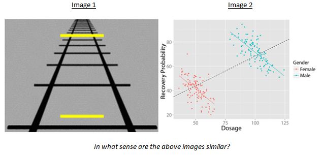
A Riddle

We begin with a riddle!

riddle

We will arrive at an answer by the end of this article. 🙂  Our journey will begin with a survey of a field within visual processing.

The Mystery Of Stereopsis

Stereopsis is the computational construction of depth from visual data. Physics is embedded in three spatial dimensions, yet your retinae are essentially 2D (imagine wrapping a sheet of paper around half of a sphere). Depth information can be gleaned from comparing the disparities between two similar images, and applying geometric principles to compute depth.  The dual images do not have to come from two eyes, either!  Close one eye, and the brain can still infer depth from motion (by comparing two images from the same eye across time).

However, stereopsis is plagued by the problem of underdetermination. The following diagram motivates this nicely:

depth_matrix

The inverse projection is your mental model of the environment. However, your brain only possesses 2D retinal images.  To recreate the environment, we consider image matches:

  1. Gray hexes are matches (left image color does not match right color)
  2. White hexes are non-matches.

The grey hexes are possible 3D interpretations of the 2D images. The black hexes are correct 3D interpretation. The brain must select a subset of grey hexes to be black hexes (which possible interpretation is veridical). This is the visual inverse problem.

The Secret To Depth Reconstruction

Visual data alone provides no obvious solution to the visual inverse problem. How then do we explain interpretation consensus (that mammals almost always agree on one particular depth-interpretation), and interpretation veracity (that the consensus is almost always correct)?

Consider the inverse projection again. Do you notice that the black hexes (correct answers) tend to be side-by-side?

In general, we might prefer interpretations (grey hexes) that are spatially continuous. The brain in fact uses cues like spatial continuity to solve the visual inverse problem.

Spatial continuity helps us begin to understand interpretation consensus. But it alone is insufficient for selecting only one possible interpretations. The brain relies on a total of six cognitive assumptions:

  1. Existence Of Surfaces: The visible world can be regarded as being composed of smooth surfaces having reflectance functions whose spatial structure may be elaborate.
  2. Hierarchical Organization: A surface’s reflectance function is often generated by a number of different processes, each operating at a different scale.
  3. Similarity: The items generated on a given surface by a reflectance-generating process acting at a given scale tend to be more similar to one another in their size, local contrast, color, and spatial organization that to other items on that surface.
  4. Spatial Continuity: Markings generated on a surface by a single process are often spatially organized – they are arranged in curves or lines and possibly create more complex patterns.
  5. Continuity Of Discontinuities: The loci of discontinuities in depth or in surface orientation are smooth almost everywhere.
  6. Continuity Of Flow: If direction of motion is ever discontinuous at more than one point – along a line, for example – then an object boundary is present.

In his book, Marr shows how these assumptions can be expressed in computational algorithms that solve the visual inverse problem. Further, neurobiological evidence suggests that one of them is the actual mechanism used by our brains.

The Nature Of Cognitive Assumptions

Why do these cognitive assumptions work? Because Earth’s photic environment features important statistical regularities. We assume similarity because most within-object visual characteristics tends to be more homogenous than that between objects.

These six assumptions also explain many optical illusion phenomena. Most optical illusions represent statistical deviations that violate our reliance on the above assumptions. For example, the depth illusion at the beginning of the article violates our our brain’s natural intuitions about perspective. Such illusions therefore are not a misfiring of an individual human vision system. It is a design consequence.

How do our brains know about these statistical regularities? Two vehicles suggest themselves:

  1. Natural Selection. Since the world is rife with statistical regularities, organisms that encode this structure more efficiently will tend to outperform their peers.
  2. Developmental Learning. In addition to short-term episodes visual inference, the visual system might itself learn to retain information about statistical regularities. This is e.g., suggested in recent research on visual normalization.

If physics were different, the statistics of everyday vision would be different, and thus a different collection of cognitive assumptions would have emerged.

Crossing The Bridge To Causal Inference

Gopnik et al suggest that cognitive assumptions are not unique to vision. Causal inference also relies on statistical regularities of causations. Specifically, the following causal assumptions are relied on by the brain:

  1. Markov Assumption. If the conditional probability distribution of future states of the process (conditional on both past and present values) depends only upon the present state; that is, given the present, the future does not depend on the past.
  2. Faithfulness Assumption. In the joint distribution on the variables in the graph, all conditional independencies are consequences of the Markov assumption applied to the graph.

The Markov assumption says that there will be certain conditional independencies if the graph has a particular structure, the faithfulness assumption says that there will be those conditional independencies only if the graph has a particular structure. The faithfulness assumption supplies the other half of the biconditional.

Solving The Riddle

Statisticians have long known about Simpson’s Paradox: “a paradox in which a trend that appears in different groups of data disappears when these groups are combined, and the reverse trend appears for the aggregate data”.

Image 2 summarizes this effect well: only when you disaggregate gender can you see the deleterious effect of the drug on recovery probability.

riddle

These two figures are similar in virtue of the fact that they violate cognitive assumptions embedded in all neurotypical adults:

  • Image 1 violate visual assumptions (perspective assumptions)
  • Image 2 violate causal assumptions (faithfulness assumption)

References

  • Marr (1982). Vision.
  • Gopnik et al (2004). A Theory of Causal Learning in Children: Causal Maps and Bayes Nets

Causal Inference with pcalg

Part Of: Causal Inference sequence
Content Summary: 2200 words, 22 min read

Introduction

In this post, we’re going to explore one way to do causal inference, as described in the following article:

Title: More Causal Inference with Graphical Models in R Package pcalg
Authors: Kalisch, K et. al
Published: 2014
Citations: 49 (note: as of 04/2014)
Link: Here (note: not a permalink)

Setting The Stage

Statistics is haunted by soundbites like few other professions. “Lies, damned lies, and statistics” needs to die. The way to mitigate deceit is not ignorance, it is the promotion of statistical literacy. “Correlation does not imply causation” should also be expunged. There must be a way to affirm the significance of spurious correlations without blinding people to the fact that causation can be learned from correlation.

When you read someone like C.S. Peirce, you will hear claims that causality is dead. Causality is, indeed, a very ancient topic. In the medieval period, the Aristotelian story about causality – a quadpartite distinction of Material Cause, Formal Cause, Efficient Cause, Final Cause – dominated the intellectual landscape. The moderns, however, were largely dissatisfied with this story; with the Newtonian introduction of forces, the above distinction began to fade into the background. So why are scientists now trying to reclaim causality from the annals of philosophy?

Enter Judea Pearl, champion of Bayesian networks and belief propagation. Dissatisfied with his near-godlike contributions to humanity, he proceeded to found modern causal theory with this text, appropriately named Causality. The reason that causality has reclaimed its sexiness is because Pearl found a way to quantize it, to update one’s beliefs about it, from raw data. Pearl grounds his version of causality in counterfactual reasoning, and borrows heavily from modal logic (c.f., possible worlds). He also introduces the notion of do-calculus, noting that there needs to exist within probability theory, operators that model action (just as “|” models observation). This SEP section explores the philosophical underpinnings of the theory in more depth.

Pearl’s movement is picking up speed. Today, you’ll find causal inference journals, conferences bent on exploring the state of the art, and business leaders trying to harness its powers to make a profit. Causal inference will be the next wave of the big data movement. It explains how human brains create concepts. It is the future of politics.

Put on your seatbelts. We’re going to take causal inference software – an R package named pcalg – out for a drive. If you want the driver’s wheel, you can have it: install RStudio, and refer to the step-by-step tutorial in the paper (or, see Appendix below). This article won’t attempt to install a complete understanding of causal models; I am content to build up your vocabulary.

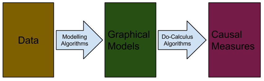
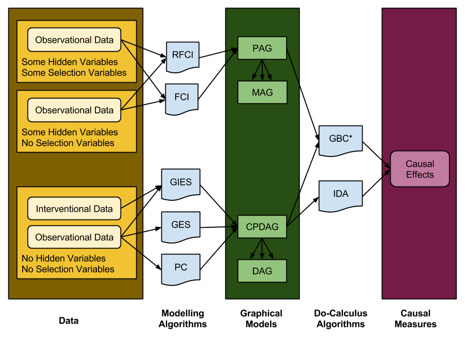
The causal inference process can thus be modeled as three causal artifacts (data, models, measures), and two algorithm categories (modelling, do-calculus).

Causal Models- Overview

Causal Artifacts

Subtleties With Data

By data we normally mean observational data, which consists of random variables that are independent and identically distributed (iid assumption). However, sometimes our algorithms must process interventional data. What is the difference?

We often have to deal with interventional data in causal inference. In cell biology for example, data is often measured in different mutants, or collected from gene knockdown experiments, or simply measured under different experimental conditions. An intervention, denoted by Pearl’s do-calculus, changes the joint probability distribution of the system; therefore, data samples collected from different intervention experiments are not identically distributed (although still independent).

How do we get from raw data to causal relationships? The secret lies in conditional independence: “Can I use this variable to predict that one, given that I know the value of this third data point?”. Specifically, conditional independence is used to infer a property known as d-separation. D-separation enables us to prune away edges that represent spurious correlations.

We only deal with distributions whose list of conditional independencies perfectly matches the list of d-separation relations of some DAG; such distributions are called faithful. It has been shown that the set of distributions that are faithful is the overwhelming majority [7], so that the assumption does not seem to be very strict in practice.

How do we learn conditional independencies? From an conditional-independence oracle, a black box that unfailingly gives us the correct answers. While such a thing is not realized in the real world, an approximation of it is, in fact, leveraged by our causal algorithms:

In practice, the conditional independence oracle is replaced by a statistical test for conditional independence. For… the PC algorithm, [this replacement] is computationally feasible and consistent even for very high-dimensional sparse DAGs.

But hold on, you may say, data does not just drop into our lap. Data in the real world is incomplete, there may be variables we simply are not tracking (hidden variables). Worse, the subset of data that materializes in front of us is often non-random, but the product of observer bias: selection variables are at work behind the scenes. As you will see, we can and we will account for these.

A Hierarchy Of Graphical Models

I will present four different types of graphical models.

A DAG (directed acyclic graph) is our language of causality. There exist only one type of edge in a DAG:

  1. Blank-Arrow. These two edgemarks together represent the direction of causation.

Let’s break down the meaning of the acronym. A DAG is:

  • directed due to its arrows
  • acyclic in virtue of the fact that you can’t follow the arrows around in a circle.
  • graphical because it has nodes and edges

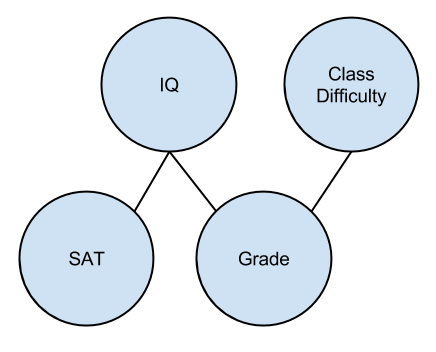
An example:

Causal Models- DAG

Notice that this diagram makes the distinction between causality and causation quite clear. SAT may be highly correlated with grade, but it has no causal effect on it. In contrast, Class Difficulty is highly correlated with Grade, and it has a causal effect on it. We tell the difference by d-separation.

Two requisite concepts before we go further.

  1. A skeleton is basically a graph with its edgemarks removed.
  2. An equivalence class is a set of graphs with the same skeleton but with different edgemarks. They are the set of all possible graphs consistent with the data.

Here’s a skeleton of our DAG:

Causal Models- DAG Skeleton

A CPDAG (completed partially directed acyclic graph) [1] is an equivalence class of DAGs. There exists two types of edges in a CPDAG:

  1. Blank-Arrow. The causal direction is displayed clearly if all members of the equivalence class agree.
  2. Arrow-Arrow. The causal direction is ambiguous if there is internal disagreement between members of the equivalence class.

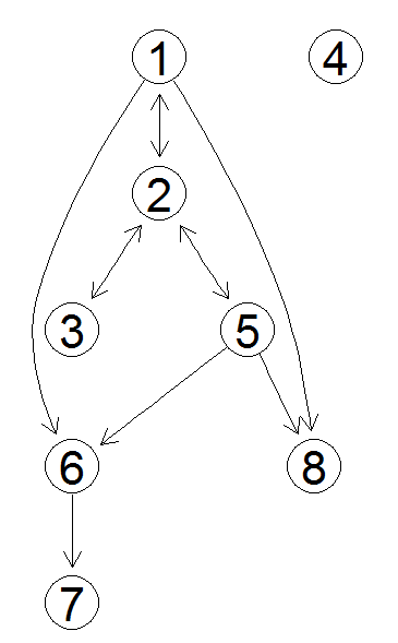
An example:

cpdag

From the above two observations, we see that all DAGs in this equivalence class agree on the V6-V7 relation, but disagree about the V1-V2 relation.

Why would we even need to even conceive of such a graph, if DAGs are enough to represent the state of the world? Because, typically, our algorithms can only produce CPDAGs:

Finding a unique DAG from an independence oracle is in general impossible. Therefore, one only reports on the equivalence class of DAGs in which the true DAG must lie. The equivalence class is visualized using a CPDAG.

But even CPDAGs cannot accommodate those pesky hidden and selection variables!

Suppose, we have a DAG including observed, latent and selection variables and we would like to visualize the conditional independencies among the observed variables only. We could marginalize out all latent variables and condition on all selection variables. It turns out that the resulting list of conditional independencies can in general not be represented by a DAG, since DAGs are not closed under marginalization or conditioning. A class of graphical independence models that is closed under marginalization and conditioning and that contains all DAG models is the class of ancestral graphs.

A MAG (maximal ancestry graph) [8] thus affords for hidden and selection variables. There exist three types of edges in a MAG:

  1. Blank-Arrow. Roughly, these edges come from observed variables.
  2. Arrow-Arrow. Roughly, these edges come from hidden variables.
  3. Blank-Blank. Roughly, these edges come from selection variables.

Let me note in passing that MAGs rely on m-separation, a generalization of d-separation.

The same [motivation for CPDAGs holds] for MAGs: Finding a unique MAG from an independence oracle is in general impossible. One only reports on the equivalence class in which the true MAG lies (a PAG).

A PAG (partial ancestry graph) [11] is an equivalence class of MAGs. There exist six kinds of edges in a PAG:

  1. Circle-Circle
  2. Circle-Blank
  3. Circle-Arrow
  4. Blank-Arrow
  5. Arrow-Arrow
  6. Blank-Blank

PAG edgemarks have the following interpretation:

  • Blank: this blank is present in all MAGs in the equivalence class.
  • Arrow: this arrow is present in all MAGs in the equivalence class.
  • Circle: there is at least one MAG in the equivalence class where the edgemark is a Blank, and at least one where the edgemark is an Arrow.

Causal Measures

Okay, let’s rewind. Suppose we are in possession of the following CPDAG (whose equivalence class consists of two DAGs):

cpdag

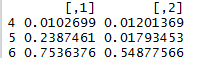
This diagram allows us to, at a glance, evaluate the relationships between variables. However, it does not address the following question: how strong are the causal relationships? Suppose we wish to quantify the causal strength V1 has over V4, V5, and V6. It turns out that this can be done with the application of Pearl’s methods (including do-calculus). With these techniques in hand, we feed this CPDAG to our do-calculus algorithm, and receive the answer!

effects

I’ll let the authors explain what this matrix means:

Each row in the output shows the estimated set of possible causal effects on the target variable indicated by the row names. The true values for the causal effect are 0, 0.0, and 0.52 for variables V4, V5 and V6, respectively. The first row, corresponding to variable V4, quite accurately indicates a causal effect that is very close to zero or no effect at all. The second row of the output, corresponding to variable V5, is rather uninformative: although one entry comes close to the true value, the other estimate is close to zero. Thus, we cannot be sure if there is a causal effect at all. The third row is [like V4 in that it is clear].

Causal inference algorithms, therefore, do not completely liberate us from ambiguity: will are still uncertain of the character of the V1-V5 relation.  But, in the V1-V4 and V1-V6 links, we see a different kind of theme: equivalence-class consensus.

Algorithm Categories

Inference Algorithms

  • The PC (Peter-Clark) algorithm [10] takes observational, complete data and outputs a CPDAG.
  • The GES (Greedy Equivalence Search) algorithm [2] performs the same function, but is faster in virtue of its greediness.
  • The GIES (Greedy Interventional Equivalence Search) algorithm [4] generalizes the GES to accommodate interventional data.
  • The FCI (Fast Causal Inference) algorithm [9] [10] accepts observational data with an arbitrary number of hidden or selection variables, and produces a PAG.
  • The RFCI (Really Fast Causal Inference) algorithm [3] does approximately the same thing, faster!

Do-Calculus Algorithms

  • The IDA (Intervention calculus when DAG is Absent) algorithm [5] accepts CPDAGs, and produces a causal measure.
  • The GBC (Generalized Backdoor Criterion) algorithm [6] is able to handle hidden variables, but cannot handle selection variables. It takes PAG, MAG, CPDAG, or DAG models and checks whether a causal measure can be estimated. If it can, it goes ahead and gathers precisely that information.

In passing, the authors note that, in [5], “IDA was validated on a large-scale biological system”.

Conclusion

The Causal Landscape

Time to tie everything together!

Causal Models- Landscape

The State Of The Art

This field is expanding very rapidly. I had the opportunity to read an earlier version of this paper in 2012. To give you a taste of the rate of change, it appears to me that the authors have both produced the mathematics for the GIES and GBC algorithm, and implemented them in R, during the intervening months.

It is useful to gauge a field’s progress in terms of theory constraint – what can we say No to, with these new methods?

  • We can say No to non-quantitative rhetoric.
  • We can say No to appeals to unconstrained ambiguity.
  • We can say No to erroneous causal skeletons.
  • We can say No to denials of equivalence-class consensus.

I have a dream that policy makers will pull up CPDAGs of, say, national economics, and use the mathematics to quantitatively identify points-of-agreement. I have a dream that the strengths of our Nos will clear away the smoke from our rhetorical battlefields long enough to find a Yes.

It is such an exciting time to be alive.

References

[1] Andersson et al (1997). “A characterization of Markov equivalence classes for acyclic digraphs”.
[2] Chickering (2002). “Optimal structure identification with greedy search”
[3] Colombo et al. (2012). “Learning High-Dimensional directed acyclic graphs with latent and selection variables”.
[4] Hauser and Buhlmann (2012). “Characterization and greedy learning of interventional Markov equivalence classes of directed acyclic graphs.”
[5] Maathius et al (2010). “Predicting Causal Effects in Large-Scale Systems from Observational Data”.
[6] Maathuis and Colombo (2013). “A generalized backdoor criterion”.
[7] Meek (1995). “Strong completeness and Faithfulness in Bayesian Networks.”
[8] Richardson and Spirtes (2002). “Ancestral Graph Markov Models”
[9] Spirtes et al (1999). “An Algorithm for Causal Inference in the Presence of Latent Variables and Selection Bias.”
[10] Spirtes et al (2000). Causation, Prediction, and Search. Adaptive Computation and Machine Learning, second edition. MIT Press, Cambridge.
[11] Zhang (2008) “On the completeness of orientation rules for causal discovery in the presence of latent confounder and selection bias”.

Appendix: Example Commands

> install.packages(“pcalg”)
> source(“http://bioconductor.org/biocLite.R”)
> biocLite(“RBGL”)
> biocLite(“Rgraphviz”)
> library(“pcalg”)
> data(“gmG”)
> suffStat pc.gmG stopifnot(require(Rgraphviz))
> par(mfrow = c(1,2))
> plot(gmG$g, main = “”) ; plot (pc.gmG, main = “”)
> idaFast(1, c(4,5,6), cov(gmG$x), pc.gmG@graph)

Modularity & The Argument From Design

Part Of: Cognitive Modularity sequence
See Also: Fodor: Modularity of Mind
Content Summary: 1600 words, 16min read

Introduction

This post represents an argument for a particular thesis, known as massive modularity. This thesis, particularly popular among evolutionary psychologists, states that the mind is rife with mental modules, and that the cognitive life is the interplay between them.

What is a mental module? If you don’t have a clear grasp on what that means, I recommend just glancing my summary of Fodorian modularity. Bear in mind, though, that here the term is used somewhat differently: modules here may be some subset of the listed properties.

The following argument is not my own, it is rather an interpretation of Carruther’s argument, which is presented in this text, under Section 1.3.

Motivators From Biology

Carruthers starts by surveying the biological literature for instances of modularity. And he finds it, by the truckload:

There is a great deal of evidence from across many levels in biology to the effect that complex functional systems are built up out of assemblies of sub-components. This is true for the operations of genes, of cells, of cellular assemblies, of whole organs, of whole organisms, and of multi-organism units like a bee colony. And by extension, we should expect it to be true of cognition also, provided that it is appropriate to think of cognitive systems as biological ones, which have been subject to natural selection.

Amongst other sources, he cites the following research:

  • West-Eberhard, 2003. Developmental Plasticity and Evolution.
  • Seeley, 1995. The Wisdom of the Hive: the social physiology of honey bee colonies.

We thus possess considerable biological reason to believe that:

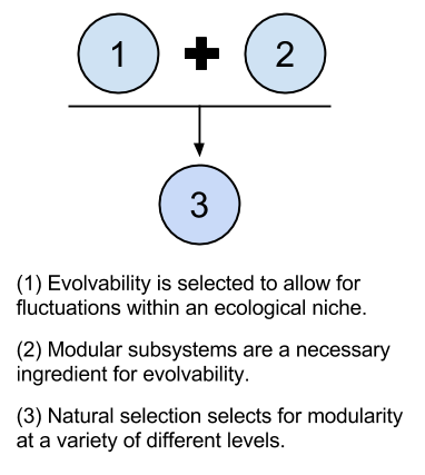
(3) Natural selection selects for modularity at a variety of different levels.

A Role For Evolvability

It’s one thing to observe natural selection promoting modularity, it is another to understand why it is doing so. To do this, we must appeal to the concept of evolvability.

Biological populations tend to conform themselves to ecological niches. That is, a species tends to adopt a particular survival strategy that exploits a certain subset of the local biosphere. Let me here decorate a concept I like to call niche distance: two species said to be in direct competition are so in virtue of the fact of short niche distance, etc. Thus, we could say that the niche distance between two types of weeds in your backyard is small, and the niche distance between the weed and the bald eagle is large.

The fact that niches change is one of the drivers for biological evolution. For example, as the earth warms in the coming centuries, mammalian species will need to acclimate to a different climate, which entails a changed vegetative response, which entails a need for change in eating patterns, etc. Such niche fluctuations are ubiquitous.

We know that evolution is driven by the engine of mutation. But mutation is simply a stochastic, quantum mechanical phenomenon:  there is no way to “speed it up”. Species typically cannot keep pace with niche fluctuations by directly modulating the rate of mutation. Rather, the genetic infrastructure of species must be able to harness mutations to keep pace with niche fluctuations. To put this concept of evolvability very crudely: natural selection does not only select for number of muscles, but also the ability to grow new ones.

(1) Evolvability is selected to allow for fluctuations within an ecological niche.

This video is a cute exploration of how evolvability may be supported in microorganisms by direct tampering of the genetic replication engine. But for larger organisms, the loci of behavior is trans-cellular. The sheer geometry of size compelled cells to become heterozygous, to constitute interdependent systems. The question of mutation containment, then, becomes central: is it possible for evolution to improve upon one function of an organism, without simultaneously affecting other functions?

Here, finally, is where modularity comes into play. One of the most important features of modularity is encapsulation: the hiding of information within specific containers. Rather than all functions affecting all other functions, computational processes erect walls around themselves, and communicate through them in a controlled fashion. Modular encapsulation is thus seen as a prerequisite for mutation containment:

(2) Modular subsystems are a necessary ingredient for evolvability.

Taken together, premise (1) and (2) support (3) in the following way:

Massive Modularity- Argument From Design- Evolvability

Motivators From Computer Science

In the above section, we were given a nice intuition regarding Premise 2: that modularity affords for mutation containment. But perhaps this intuition can be buffered with evidence from somewhere else entirely:

The basic reason why biological systems are organized hierarchically in modular fashion is a constraint of evolvability. Evolution needs to be able to add new functions without disrupting those that already exist; and it needs to be able to tinker with the operations of a given functional sub-system – either debugging it, or altering its processing in response to changes in external circumstances – without affecting the functionality of the remainder. Human software engineers have hit upon the same problem, and the same solution.

Two of the most widely used languages nowadays are C++ and Java. Languages in this class are often described as ‘object-oriented’. Many programming languages now require a total processing system to treat some of its parts as ‘objects’ which can be queried and informed, but where the processing that takes place within those objects isn’t accessible elsewhere. This enables the code within the ‘objects’ to be altered without having to make alterations in code elsewhere, with all the attendant risks that this would bring; and it likewise allows new ‘objects’ to be added to the system without necessitating wholesale re-writings of code elsewhere. And the resulting architecture is regarded as well nigh inevitable (irrespective of the programming language used) once a certain threshold in the overall degree of complexity of the system gets passed.

Interestingly, since the need for modular organization increases with increasing complexity, we can predict that the human mind will be the most modular amongst animal minds. This is the reverse of the intuition shared by many philosophers and social scientists, who would be prepared to allow that animal minds might be organized along modular lines, while believing that with the appearance of the human mind most of that organization was somehow superseded and swept away.

We extract the following argument from the above appeal to object-oriented programming (OOP):

(4) Software engineering suggests that OOP (modularization) is necessary to manage increasing complexity.
(5) Biological systems are very complex.

These premises buffer our Premise 2.

(2) Modular subsystems are a necessary ingredient for evolvability.

Massive Modularity- Argument From Design- OOP

I particularly enjoyed the originality of this argument. Even though software engineering is notoriously bad at quantifying its practices, its trajectory surely sheds some light on other disciplines. As a computer scientist, this argument made me speculate what other trends, current or future, could be brought to bear on such questions. The interchange between computer science and cognitive neuroscience is broad… with things like neuromorphic computing flowing in one direction, and information theory flowing in the other…

Is Mind Subject To Natural Selection

This phase of the argument is the most philosophical. The question is whether mental processes are subject to the forces of natural selection.

Carruthers begins with a fairly uncontroversial premise:

(6) The central nervous system is subject to natural selection.

So much, so obvious. But the crux of the issue is how to relate mind and brain. Carruthers wants to argue that:

(7) The central nervous system underwrites the mind.

However, this premise falls squarely into a philosophy of mind morass. Carruthers suggests a way forward is to notice that most mainstream approaches (“anyone who is neither an an epiphenomenalist nor an eliminativist about the mind”) support such a premise (see this post for some definitions).

If we find ourselves sympathetic to 7, we are led by the nose to Proposition 8:

(8) Mental processes are subject to natural selection.

Massive Modularity- Argument From Design- Mental Evolution

How Many Minds

While the weight of this argument labors to support the reality of computational modules, we must also spare some words to motivate massive modularity. Carruthers, leveraging Simon, H’s 1962 paper The Architecture of Complexity, points out that the question is one of degrees. Let us try to imagine a modularity thesis that is non-massive:

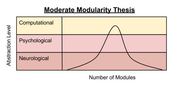
Moderate Modularity

The x-axis captures number of modules, the y-axis leverages David Marr’s concept of Tri-Level Analysis.  The concave shape of the curve represents the claim that, while the number of neurological functions may be large, the number of computational processes (e.g., belief, desire, motivation) is small.

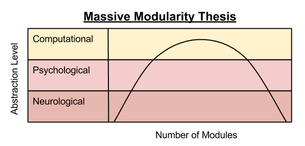
In contrast, the shape of massive modularity thesis is convex:

Massive Modularity

While Carruthers elsewhere motivates massive modularity by way of task analysis and ethological surveys, he here defends this latter thesis by appealing to the empirically-robust observation that the brain appears to process its algorithms in parallel, and this would be impossible without a relatively plentiful number of processing units. So we have stumbled upon our last premise:

(9) In the mind, massive modularity is computationally superior to moderate modularity.

Putting It All Together

All that remains is to glue together the sub-conclusions of the above arguments. Specifically, take the following propositions:

(3) Natural selection selects for modularity at a variety of different levels.
(8) Mental processes are subject to natural selection.
(9) Within the mind, massive modularity is computationally superior to moderate modularity.

From these, it is clear we have successfully motivated our thesis:

(10) Natural selection selects for massive modularity in the mind

The entire argument, then, is pictured below.

Massive Modularity- Argument From Design- Summary

Concluding Thoughts

While I happen to affirm Premise 8, I feel like Carruthers – and even more so myself – do a poor job at motivating it. This observation is particularly painful because it is arguably the central thesis of evolutionary psychology. Mental note-to-self: revisit that section of the argument.

All told, I find this argument fairly compelling, although I would like to get more clear on several of its distinctions.

Peirce: The Fixation Of Belief

[ Parent Index ]

Metadata

Article: The Fixation of Belief
Author: C.S. Peirce
Published: 11/1877
Citations: 1048 (note: as of 04/2014)
Link: Here (note: not a permalink)
Other Resources: Outline (found this via Google Search, but quality isn’t bad)

Summarization text is grayscale, review text (my take) is orange.

Preliminaries

Peirce kicks off this article with a historical survey, nicely showcasing the fact that the scientific enterprise is a quite recent phenomenon on this earth. This suggests that the construction of personal epistemologies is susceptible to cultural influences. As Peirce puts it, “We come to the full possession of our power of drawing inferences, the last of all our faculties; for it is not so much a natural gift as a long and difficult art.”

Peirce also gestures towards the following question: can the reliability of our faculties be evaluated on a domain-by-domain basis? Peirce invokes evolutionary theory in an important move:

Logicality in regard to practical matters is the most useful quality an animal can possess, and might, therefore result from the action of natural selection; but outside of these it is probably of more advantage to the animal to have his mind filled with pleasing and encouraging visions, independently of their truth; and thus, upon unpractical subjects, natural selection might occasion a fallacious tendency of thought.

While many of Peirce’s views on evolution show their age, this particular insight is remarkably prescient: modern philosophers are currently exploring precisely this vein. Once this research is cast to cognitive science, neuroscientists will find themselves in a position to speak quantitatively on the matter. If the above argument is born out by data, this would be a real victory for the pragmatist camp.

Doubt vs. Belief

Doubt is a singularly important notion to Peirce: he conceives it as the primary motivator for critical thinking.

Doubt is an uneasy and dissatisfied state from which we struggle to free ourselves and pass into the state of belief; while the latter is a calm and satisfactory state which we do not wish to avoid, or to change a belief to anything else. On the contrary, we cling tenaciously, not merely to believing, but to believing just what we do believe.

The self-preservation of belief is of particular interest to me. This phenomenon is explored in detail within social psychology and memetics.

The irritation of doubt causes a struggle to attain a state of belief. When doubt ceases, mental action on the subject comes to an end.

With this definition of doubt in place, Peirce goes on to rebut three erroneous conceptions of proof:

  1. The mere putting of a proposition into the interrogative form does not stimulate the mind to any struggle after belief. There must be a real and living doubt, and without this all discussion is idle.
  2. The premises of an argument need not be grounded in some firm metaphysical strata: they merely should be free from doubt.
  3. There is, then, no practical value in arguing a point after all the world is fully convinced of it.

This contextual backdrop resonates with anyone who has tried to persuade someone not subject to real and living doubt. There are times when words move the human heart, and times when they are “just words”. However, I am largely disappointed in this dichotomy as it stands. Questions concerning what underlies, motivates, or justifies doubt are unattended. Peirce may not have been in an empirical position to cognitively explain doubt, but surely he could have afforded to provide a more detailed sketch.

Peirce goes on to detail four methods for the fixation of belief. I will summarize each in turn.

Belief Fixation Method #1: Method of Tenacity

Peirce uses examples to shed light on this way of being:

I remember once being entreated not to read a certain newspaper lest it might change my opinion upon free-trade. “Lest I might be entrapped by its fallacies and misstatements,” was the form of expression. “You are not,” my friend said, “a special student of political economy. You might, therefore, easily be deceived by fallacious arguments upon the subject. You might, then, if you read this paper, be led to believe in protection. But you admit that free-trade is the true doctrine; and you do not wish to believe what is not true.” A similar consideration seems to have weight with many persons in religious topics, for we frequently hear it said, “Oh, I could not believe so-and-so, because I should be wretched if I did.” A man may go through life, systematically keeping out of view all that might cause a change in his opinions…

How, then, are we to evaluate such a method?

It would be an egotistical impertinence to object that his procedure is irrational, for that only amounts to saying that his method of settling belief is not ours. But this method of fixing beliefs will be unable to hold its ground in practice. The man who adopts it will find that other men think differently from him, and it will be apt to occur to him, in some saner moment, that their opinions are quite as good as his own, and this will shake his confidence in his belief. This conception, that another man’s thought or sentiment may be equivalent to one’s own, is a distinctly new step, and a highly important one.

Yes! In my language, I call this Symmetry Debiasing. I intend to write more on this; it has played a role in my own worldview maturation.

Now, this first method is typically localized to the individual. The second method solves the problem of socializing belief acquisition.

Belief Fixation Method #2: Method of Authority

Here, belief is a group activity. Doxastic content is something one inherits, and its contents are to be trusted.

Uniformity of opinion will be secured by a moral terrorism to which the respectability of society will give its thorough approval. Following the method of authority is the path of peace. Certain non-conformities are permitted; certain others (deemed unsafe) are forbidden. These are different in different countries and in different ages; but, whoever you are, let it be known that you seriously hold a tabooed belief, and you may be perfectly sure of being treated with a cruelty less brutal but more refined than hunting you like a wolf.

Evidence for this sort of thing is ubiquitous; with political infighting serving as a nice example.

Thus, the greatest intellectual benefactors of mankind have never dared, and dare not now, to utter the whole of their thought; and thus a shade of prima facie doubt is cast upon every proposition which is considered essential to the security of society.

I like to play a game when I read pre-modern philosophers discuss religion: count the number of sentences wasted in defensive posturing “always remember that when I say X I do not mean Y”. Keeping your eye tuned to this kind of historical artifact, which I call the Placating Price, is a good heuristic for approximating the degree of fear behind the artful prose of the academic. And it has been considerable. Reviewing the posthumous publication of Hume’s Dialogues Concerning Natural Religion underscores this point nicely.

For the mass of mankind, then, there is perhaps no better method than this. If it is their highest impulse to be intellectual slaves, then slaves they ought to remain.

Fighting words.

Belief Fixation Method #3: A Priori Method

Systems of this sort have been chiefly adopted because their fundamental propositions seemed “agreeable to reason”. This is an apt expression; it does not mean that which agrees with experience, but that which we find ourselves inclined to believe. Plato, for example, finds it agreeable to reason that the distances of the celestial spheres from one another should be proportional to the different lengths of strings which produce harmonious chords. Many philosophers have been led to their main conclusions by considerations like this…

This method is far more intellectual and respectable from the point of view of reason than either of the others… but its failure has been the most manifest. It makes of inquiry something similar to the development of taste; but taste, unfortunately, is always more or less a matter of fashion.

Philosophy has acquired a poor reputation in many intellectual circles for precisely this reason. Certain strains of metaphysics constitute, arguably, Diseased Disciplines. Peirce also manages to anticipate modern arguments towards the refactoring of analytic philosophy.

Belief Fixation Method #4: Scientific Method

Peirce goes on to sketch a method familiar to our modern ears: the scientific method.

20071210_ScientificMethod

He also makes the interesting move in tying the method to scientific realism (the belief that things like atoms really exist, are really embedded in spacetime). His defense of scientific realism is as follows

It may be asked how I know that there are any Reals. The reply is this:

  1. If investigation cannot be regarded as proving that there are Real things, it at least does not lead to a contrary conclusion; but the method and the conception on which it is based remain ever in harmony. No doubt of the method, therefore, arise from its practice, as is the case with all the others.
  2. The feeling which gives rise to any method of fixing belief is a dissatisfaction at two repugnant propositions. But here already is a vague concession that there is some one thing which a proposition should represent. Nobody, therefore, can really doubt that there are Reals, for, if he did, doubt would not be a source of dissatisfaction. The hypothesis, therefore, is one which every mind admits. So that the social impulse does not cause men to doubt it.
  3. Everyone uses the scientific method about a great many things, and only ceases to use it when he does not know how to apply it.
  4. Experience of the method has not led us to doubt it, but on the contrary, scientific investigation has had the most wonderful triumphs in the way of settling opinion. These afford the explanation of my not doubting the method or the hypothesis which it supposes; and not having any doubt, nor believing that anybody else whom I could influence has, it would be the merest babble for me to say more about it.

If there be anybody with a living doubt upon the subject, let him consider it.

Peirce and I even share a similar sense of humor. 🙂 I love this parody of Mark 4:23!

Concluding Thoughts

After reading this essay, I do not see myself walking around and categorizing people with Method 1, 2, 3, or 4 (nor even some linear superposition of all four). I am simply not persuaded that these epistemological preferences represent natural kinds.

One might imagine combining Methods 3 and 4, and then casting the three resultant categories to personal dispositions: one based on fear/simplicity/opportunism, another on social belonging, a third on the need for cognition. With this tripartite division of epistemology based on disposition, one could then layer on cultural distinctions, such as intuitive vs quantitative philosophizing. But even this, more sophisticated, account doesn’t feel precise enough for my liking.

Why spend time on this essay if I don’t agree with its central thesis? For one, it brings key questions to the fore:

  • How does doubt affect belief construction?
  • How do individuals go about constructing personal epistemologies?

But, more importantly, the journey to our destination was interesting.

I’ll close with Peirce explaining his preference for the scientific method.

Yes, the methods [besides the scientific method] do have their merits: a clear logical conscience does cost something – just as any virtue, just as all that we cherish, costs us dear. But we should not desire it to be otherwise. The genius of a man’s logical method should be loved and reverenced as his bride, whom he has chosen from all the world. He need not condemn the others; on the contrary, he may honor them deeply, and in so doing only honors her the more. But she is the one that he has chosen, and he knows that he was right in making that choice. And having made it, he will work and fight for her, and will not complain that there are blows to take, and will strive to be a worthy knight and champion of her from the blaze of whose splendors he draws his inspiration and his courage.

A man on fire…

[ Parent Index ]