
Part Of: Algebra sequence
Followup To: Eigenvalues and Eigenvectors
Content Summary: 1300 words, 13 min read.
Limitations of Eigendecomposition
Last time, we learned how to locate eigenvalues and eigenvectors of a given matrix. Diagonalization is the process where a square matrix can be decomposed into two factors: a matrix 

But as we saw with the spectral theorem, eigendecomposition only works well against square, symmetric matrices. If a matrix isn’t symmetric, it is easy to run into complex eigenvalues. And if a matrix isn’t square, you are out of luck entirely!

Can we generalize eigendecomposition to apply to a wider family of matrices? Can we diagonalize matrices of any size, even if they don’t have “nice” properties?
Yes. Self-transposition is the key insight of our “eigendecomposition 2.0”. We define the self-transpositions of 


Suppose 


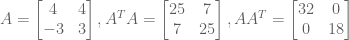
To illustrate, consider the following.

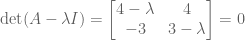
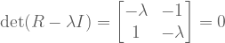
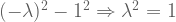
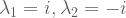
Since A is not symmetric, we have no guarantee that its eigenvalues are real. Indeed, its eigenvalues turn out to be complex:


Eigendecomposition on
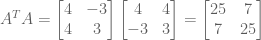

These matrices are symmetric! Thus, they are better candidates for eigendecomposition.
Towards Singular Value Decomposition
Singular Value Decomposition (SVD) is based on the principle that all matrices are eigendecomposable after self-transposition. It is essentially a bug fix:

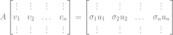
An important way to picture SVD is with the idea of orthogonal bases. It is relatively easy to find any number of orthogonal bases for a given rowspace. Call the matrix of orthogonal vectors 
We desire to find an orthogonal basis 

We won’t require vectors in
As we will soon see, these scaling factors are not eigenvalues. Instead, we will use sigmas instead of lambdas.
- Scaling factors
, analogous to eigenvalues
.
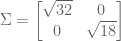
- Diagonal matrix
, analogous to diagonal matrix
Our full picture then, looks like this:

Let us now translate this image into matrix language.
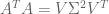
But we can easily factorize the right-hand side:

So we have that:

Since both

This strongly resembles our diagonalization equation 
Recalling that 

But now the innermost term cancels. Since 
Since

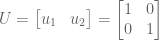
To find

The relationships between SVD and eigendecomposition are as follows:
If any eigenvalue is negative, the corresponding sigma factor would be complex. But 

In contrast to eigendecomposition, every matrix has an SVD decomposition. Geometrically,

A Worked Example
Let’s revisit
Eigendecomposition against


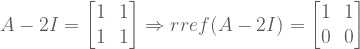
These are positive, real eigenvalues. Perfect! Let’s now derive the corresponding (normalized) eigenvectors.


SVD intends to decompose 

What’s missing?

We have arrived at our first Singular Value Decomposition.

Okay, so let’s check our work. 😛

These matrices are a viable factorization: multiplication successfully recovers
Takeaways
- Eigendecomposition only works for a subclass of matrices; SVD decomposes all matrices.
- SVD relies on self-transposition to convert any arbitrary matrix into one that works well against eigendecomposition (guarantees square
and symmetric
).
- Another way to interpret SVD is by taking a special kind of orthogonal basis that, once passed through the linear transformation, preserves its orthogonality.
- Every matrix
. That is, every linear transformation can be conceived as rotation + scaling + rotation.
Until next time.
 degrees.
 whose output vectors
  differ by a scaling factor.
 ).
).
 pairs that satisfy the above equality.
 matrix, there are
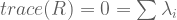
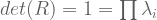
  eigenvalues. These eigenvalues can be difficult to find. However, two facts aid our search:
 from both sides:
 has an empty nullspace, it will contain zero eigenvectors. So we desire this new matrix to be singular.
 . Matrices are singular iff their determinants equal zero.


 :
:

 :
:


 ?
?
![A = \left[ \begin{smallmatrix} 3 & 1 \\ 1 & 3 \\ \end{smallmatrix} \right]](https://s0.wp.com/latex.php?latex=A+%3D+%5Cleft%5B+%5Cbegin%7Bsmallmatrix%7D+3+%26+1+%5C%5C+1+%26+3+%5C%5C+%5Cend%7Bsmallmatrix%7D+%5Cright%5D&bg=ffffff&fg=555555&s=0&c=20201002) has real eigenvalues, but
has real eigenvalues, but ![R = \left[ \begin{smallmatrix} 0 & -1 \\ 1 & 0 \\ \end{smallmatrix} \right]](https://s0.wp.com/latex.php?latex=R+%3D+%5Cleft%5B+%5Cbegin%7Bsmallmatrix%7D+0+%26+-1%C2%A0%5C%5C+1+%26+0%C2%A0%5C%5C+%5Cend%7Bsmallmatrix%7D+%5Cright%5D&bg=ffffff&fg=555555&s=0&c=20201002) has less-desirable complex eigenvalues.
has less-desirable complex eigenvalues. as follows:
 . What happens when you multiply the original matrix


 . Thus, if
 :
:
 :
:
 What is
  ?
?

 .
.


 and
and  . We can then express the Fibonnaci matrix


 is always smaller than
  , because we know all variables are positive. So we have an upper bound OPT ≤ 6. We can sharpen this upper bound, by comparing the objective function to other linear combinations of the constraints.
 . What values of these variables give us the smallest upper bound? Importantly, this is itself an objective function:
 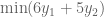 .
. and
and  are constrained: they must produce an equation that exceeds


 and
and 


 . But this is not always the case. In fact, the optimal dual value can be smaller .


 that can assume discrete values
  . Our partial understanding of the processes which determine
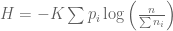
  . We would like to find some
  , which measures the uncertainty of this distribution.
 by combining events x2 and x3.

 and
and  . The uncertainty of two distributions is the sum of each individual uncertainty. Thus we add H(⅔, ⅓). But this distribution is reached only ½ of the time, so we multiply by 0.5.
 ? Consider a new
  , by definition.
  . Then we have:
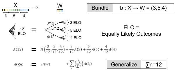
 . This simplifies things:
 hold? There is only one solution, as shown in Shannon’s paper:
 varies with logarithmic base (bits, trits, nats, etc). With this solution we can derive a general formula for entropy
  .
.

 )
) ← Found by arbitrary bundling (eg.,
  )
)
![K \left[ \sum{p_i \log(\sum{n_i})} - \sum{p_i \log(n_i)} \right]](https://s0.wp.com/latex.php?latex=K+%5Cleft%5B+%5Csum%7Bp_i+%5Clog%28%5Csum%7Bn_i%7D%29%7D+-+%5Csum%7Bp_i+%5Clog%28n_i%29%7D+%5Cright%5D&bg=ffffff&fg=555555&s=0&c=20201002)


 , where


 :
:

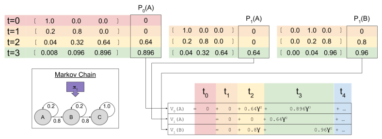
 look familiar? That’s because it equals
  ! In this way, we have a way of equating a valuation at t=0 and t=1. This property is known as intertemporal consistency.
 . Let’
 and
and  . If you fix
  you can uniquely represent

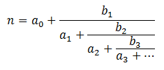
 with four coefficients. It turns out that every rational number can be expressed with a finite number of leading coefficients.


 ? It repeats, of course! What is the repeating sequence for
  ? The sequence
  .
. ? Well, after the first two digits, we notice an interesting pattern
  then
then  then
then  . The value of this triplet is non-periodic, but easy enough to compute. The situation looks even more bleak when you consider the
  …
… (golden ratio) and
  feature repeating coefficients, but
  and
and  (Euler’s number) do not. What differentiates these groups?
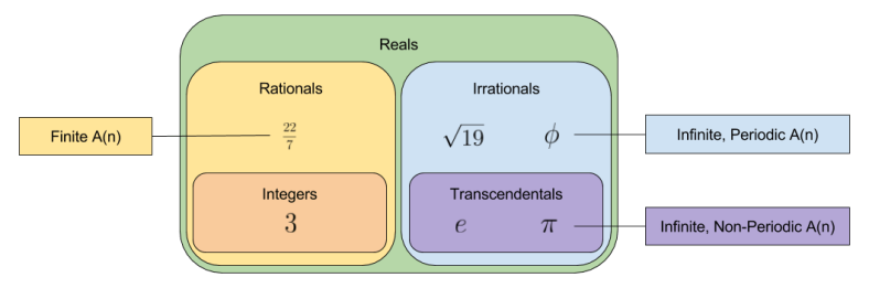
 is surprisingly close:


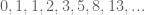
 . Here is a graph of the first two hundred:
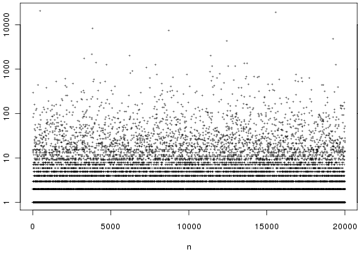

 . Here only
