
Part Of: Information Theory sequence
Content Summary: 1000 words, 10 min read
History of Communication Systems
Arguably, three pillars of modernity are: industrialization, democratic government, and communication technology. Today, we examine the latter.
Before 1860, long-distance communication required travel. This made communication across large nations quite challenging. Consider, for example, the continental United States. In 1841, it took four months for the news of the death of President Harrison to reach Los Angeles.
The Pony Express (a mail service built on horsepower) improved wait times to ten days. But it was the telegraph that changed the game. The key idea was to send messages on paper, but rather through voltage spikes in electric cables. Electrical pulses travel at near the speed of light.
In 1861, the first transcontinental cable was complete, and instantaneous communication became possible. The Pony Express closed its doors two days later.
It is hard to understate the impact of this technology. These advances greatly promoted information sharing, economic development, and improved governance.
By 1891, thousands of miles of cable had been lain underwater. These pipelines have only become more numerous and powerful over the years. Without them, the Internet would simply be impossible.

Today, we strive to understand the maths of communication.
Understanding Communication
We start with the basics.
What is communication? The transmission of linguistic information.
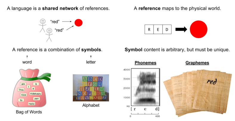
What is language? A shared system of reference communicated through symbols.
References (e.g., words) are functions that maps itself to an aspect of the physical world. References can denote both objects and actions.
Consider the power set of symbols (all possible combinations of letters). Words represent a subset of this object (a family of sets over an alphabet).
Symbol recognition is medium independent. For example, a word can be expressed either through writing (graphemes) or spoken language (phonemes).
References are the basis of memory. They together build representations of the physical world.
All complex nervous systems construct references. Some animals can communicate (share references). Only humans do so robustly, via syntax.
Semantic interpretations are not restricted to biology. Computers can refer as well. Reference is made possible by symbol grounding.
As the substrate of reference, symbols are the basis of computation. All answerable questions can be solved by a Turing machine.
Semantic aspects of communication are irrelevant to the engineering problem. Coding theory studies symbol sets (alphabets) directly.
Comparing Alphabets
How to compare languages? Let’s find out!
There are 26 symbols in the English alphabet. How many possible three-letter words are there? The answer is 26^3 = 17,576 possible words. More generally:
Possible Messages (M) = Alphabet Size (a) ^ Number of Symbols (X)
M = aX
Log(M) = Loga(X)
Information is the selection of specific words (“red”) from the space of possible words.
We might be tempted to associate information with W. But we desire information to scale linearly with length. Two books should contain twice as much information as one. So we say information is log(M).
I(X, a) = Loga(X)
Alphabet size (logarithmic base) is not very important in this function. Suppose we choose some other base B instead. We can compare alphabets by converting logarithmic base.
Base Conversion: Logb(X) = Loga(X) / Loga(b)
I(X, a) = Loga(X) = Logb(a) * Logb(X)
I(X) = K Logb(X) where K equals Logb(a)
I(X) is known as Shannon information.
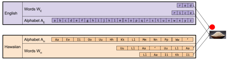
We can compare the expressive power of different alphabets. The modern Hawaiian alphabet, for example, has 13 letters. So there are only 13^3 = 2,197 possible three-letter Hawaiian words. The information provided by these respective languages is:
I(Xhawaiian) = Log13(X)
I(Xenglish) = Log13(26) * Log13(X)
I(Xenglish) / I(Xhawaiian) = Log13(26) = 1.270238
We expect English words to be 27% more information than Hawaiian, on average. And indeed, this is precisely what we find:
With 3 English letters: 26^3 = 17,576 possible words
With 3.81 Hawaiian letters: 13^(3*1.270238) = 17,576 possible words
Translating Between Codes
How does one translate between languages? Consider the word “red”. In Hawaiian, this word is “ula’ula”. We might construct the following function:
- r → ula’
- e → ul
- d → a
But this fails to generalize. The Hawaiian word for rice is “laiki”, which does not begin with a ‘u’.
In general, for natural languages any function f: AE → AH is impossible. Why? Because words (references) map to physical reality in arbitrary ways. Two natural languages are too semantically constrained to afford a simple alphabet-based translation.
Alphabet-based translations are possible, however, if you use a thin language. Thin languages only refer when converted back into its host language. Binary is a classic example of a thin language. It has the smallest possible alphabet (size two).
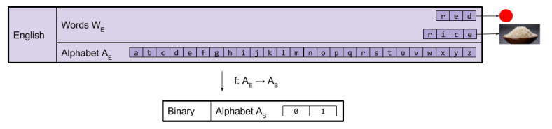
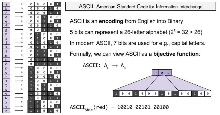
An encoding is a function of type f: AE → AH. For an example, consider ASCII. This simple encoding is at the root of most modern technologies (including UTF-8, which you are using to view this webpage):
Noise and Discriminability
A communication system has five components: source, transmitter, channel, receiver, and destination.
A source and destination typically share a common system of reference. Imagine two people with the same interpretation of the word “red”, or two computers with the same interpretation of the instruction “lb” (load byte).
Transmitter and receiver also tend to play reciprocal roles. Information is exchanged through the channel (e.g., sound waves, cable).
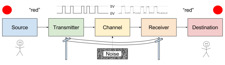
Receivers reconstruct symbols from the physical medium. Noise causes decoding errors.
How can the transmitter protect the message from error? By maximizing the physical differences between symbols. This is the discriminability principle.
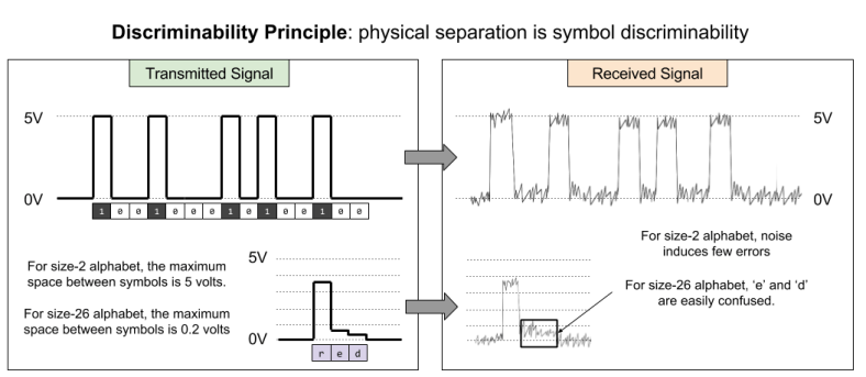
This principle explains why binary is employed by computers and telecommunications. A smaller alphabet improves symbol discriminability, which combats the effect of noise.
Takeaways
- Language is a shared system of reference communicated through symbols
- References are functions that maps itself to an aspect of the physical world.
- Symbol recognition is medium independent.
- Alphabet size determines expressive power (how many messages are possible)
- An encoding lets you alter (often reduce) language’s alphabet.
- Such encodings are often desirable because they protect messages from noise.


 that can assume discrete values
  . Our partial understanding of the processes which determine
  . We would like to find some
  , which measures the uncertainty of this distribution.
 by combining events x2 and x3.

 and
and  . The uncertainty of two distributions is the sum of each individual uncertainty. Thus we add H(⅔, ⅓). But this distribution is reached only ½ of the time, so we multiply by 0.5.
 ? Consider a new
  , by definition.
  . Then we have:
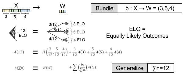
 . This simplifies things:
 does
does  hold? There is only one solution, as shown in Shannon’s paper:
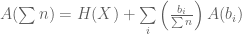
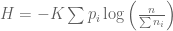
 varies with logarithmic base (bits, trits, nats, etc). With this solution we can derive a general formula for entropy
  .
.

 )
) ← Found by arbitrary bundling (eg.,
  )
)
![K \left[ \sum{p_i \log(\sum{n_i})} - \sum{p_i \log(n_i)} \right]](https://s0.wp.com/latex.php?latex=K+%5Cleft%5B+%5Csum%7Bp_i+%5Clog%28%5Csum%7Bn_i%7D%29%7D+-+%5Csum%7Bp_i+%5Clog%28n_i%29%7D+%5Cright%5D&bg=ffffff&fg=555555&s=0&c=20201002)


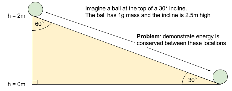
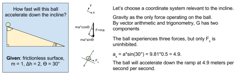
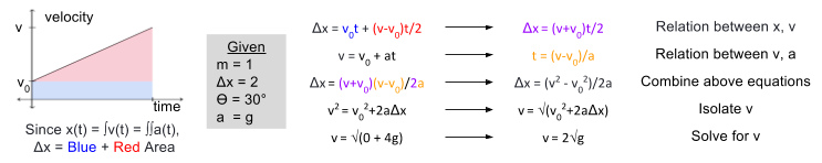
 meters per second
  m/s). However, recall the classical definitions of kinetic and potential (gravitational) energy, which are
  and
and  .
.
![m[(0 + 2g) - (\frac{ \sqrt{(4g)^2} }{2})] + 0 = m[2g - 2g] = 0](https://s0.wp.com/latex.php?latex=m%5B%280+%2B+2g%29+-+%28%5Cfrac%7B+%5Csqrt%7B%284g%29%5E2%7D+%7D%7B2%7D%29%5D+%2B+0+%3D+m%5B2g+-+2g%5D+%3D+0&bg=ffffff&fg=555555&s=0&c=20201002)
 ? Because it is experiencing a force.
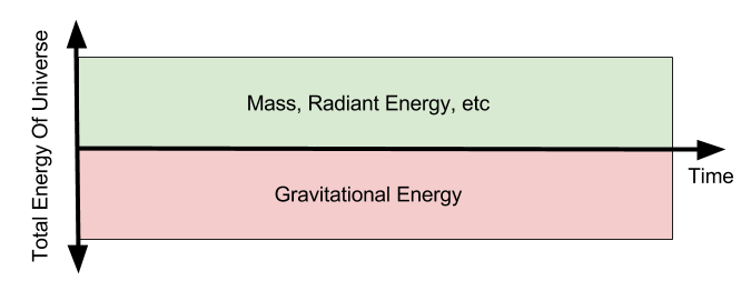


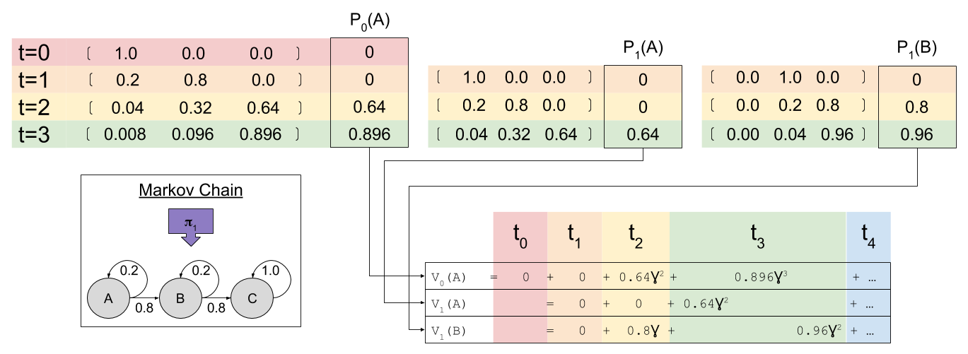
![\Delta_t = \left[ r_t(A) + \gamma \sum P(s'|s)V_{t+1}(s') \right] - V_t(s)](https://s0.wp.com/latex.php?latex=%5CDelta_t+%3D+%5Cleft%5B%C2%A0r_t%28A%29+%2B+%5Cgamma+%5Csum+P%28s%27%7Cs%29V_%7Bt%2B1%7D%28s%27%29+%5Cright%5D+-+V_t%28s%29&bg=ffffff&fg=555555&s=0&c=20201002)


 either
  or
or  or
or 
 if
if  then
then 
 then
then  s.t.
s.t.  iff
iff 
 over
over  , mixing both with the same third lottery
  in the same proportion α must not reverse that preference—adding identical “padding” is irrelevant to the choice.


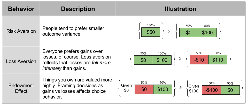
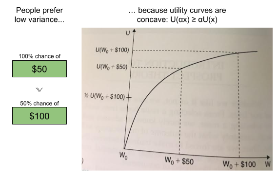
 concavity to explain risk aversion? Prospect theory takes this approach yet further, and seeks to explain all of the above behaviors using a more complex shape
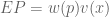
 represent our updated notion of utility. We can define expected prospect
  of a function as probability multiplied by the value function

 :
: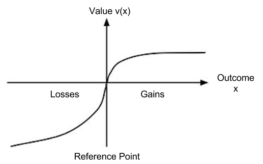
 , captures the status quo. Thus, the reference point allows us to differentiate gains and losses, thereby producing the endowment effect.

 has the following shape:
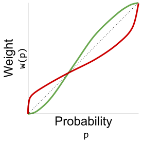


 , where


 :
:
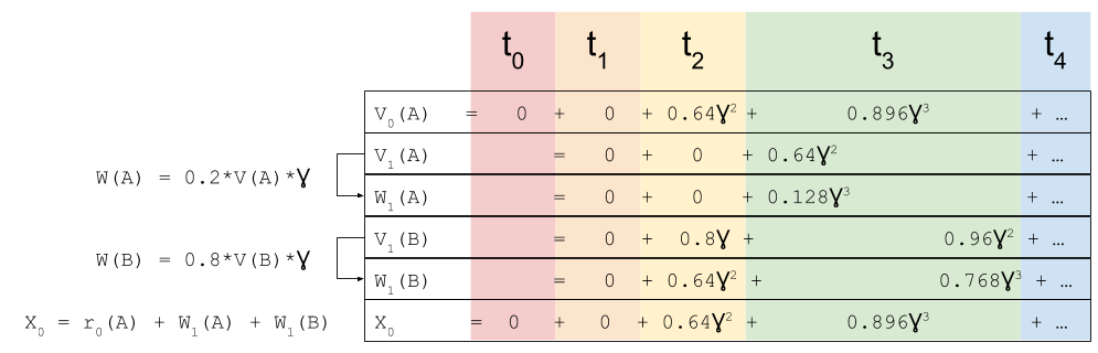
 look familiar? That’s because it equals
  ! In this way, we have a way of equating a valuation at t=0 and t=1. This property is known as intertemporal consistency.
 . Let’
