Potential Outcome Models

Part Of: Causal Inference sequence
Content Summary: 800 words, 8 min reading time

Counterfactuals

Imagine you are a doctor investigating the effects of a new drug for cancer treatment:

  • A large number of patients enroll in the trial.
  • For each patient, you may administer the drug, or a placebo.
  • For each patient, you record whether the outcome is death or survival (cancer remission).

Let’s sharpen the above account by defining variables across it:

  • N patients enroll in the trial.
  • Let X represent applied treatment. Placebo application is X=0; drug application is X=1.
  • Let Y represent patient outcome. Patient death is Y=0; patient survival is Y=1.

How many patients should we give the drug to? If we give the placebos to all patients, and all of them die, does that mean that our drug works? Of course not! Next, consider the situation where we give the drug to all patients, and all of them live. May we now conclude that the drug is effective in this scenario? Not necessarily: perhaps we have simply encountered a particularly lucky group of human beings.

Imagine next a world where we could acquire answers to any question we dare ask. Here, how would you go about determining the causal effect of our drug?

If a patient dies via the placebo, wouldn’t it be nice if we could rewind time, and observe whether the drug saved their lives (see whether the drug helps this individual)? If a patient dies via the drug, wouldn’t it be nice if we could rewind time and see whether they die via the placebo (perhaps they are beyond help)? In an ideal world, we could rewind time and acquire answers to such what if questions.

For formal name for what-if models of causality are known as counterfactuals. And counterfactual theories of causation are just one location is a vast, turbulent landscape of the West’s struggle over causation. The first time I wandered into Wikipedia’s survey of causal reasoning, my head was throbbing for hours. But let me spare you an attempt to make sense out of the philosophical implications of counterfactuals, and merely paint a formalism.

An Outcome Taxonomy

We require two more variables:

  • Let Y0 represent patient outcome after placebo administration.  Thus,  Y0=1 means placebo patient lives.
  • Let Y1 represent patient outcome after drug administration. Thus, Y1=0 means drugged patient dies.

There are only four possible types of patient:

Potential Outcomes- Drug Response Types (1)

Translating back into English:

  1. Patients of type “Never Recover” will die if given the drug, but will also die if given a placebo.
  2. Patients of type “Helped” will survive if given the drug, but will die if given a placebo.
  3. Patients of type “Hurt” will die if given the drug, but will live if given a placebo.
  4. Patients of type “Always Recover” will live if given the drug, but will also live if given a placebo.

The Machinery Of Possibility

Imagine you are omniscient, and have access to a counterfactual table of possible outcomes. That is, for either possible world (the one where you hand me a drug, and the one where you hand me a placebo), you know whether I beat my cancer. You can then generate predictions as follows:

Potential Outcomes- Model Prediction (1)

The left table is one of counterfactuals, the right is composed of observables. The X column represents a selector; it selects which column of the counterfactual table from which to draw the value of Y (X=1 means right column, X=0 means left). Pay attention to the color red, until the above makes sense.

Now let’s relax the problem and admit that we are not omniscient: scientists simply do not possess privileged access to the multiverse. Rather, you simply observe outcomes of individuals. In this world, inference moves from right-to-left, and half of all counterfactual entries are left indeterminate.

Potential Outcomes- Empirical Learning

As you can see, these indeterminate counterfactuals on the left means that the patient of that row is of indeterminate type. If a patient dies after using the placebo (second row), we do not know whether she would Never Recover, or if she would have been Helped by the drug!

Mechanized Outcome Constraint

Pay attention to the color patterns in the above image. Could you have predicted that particular pattern? I couldn’t; they feel mysterious.

If you notice your confusion, you are more likely to expend effort to dissolve it.  Patterns emerge after the following process:

Potential Outcomes- Observations vs Outcome Type

Please take a minute to come to terms with the above diagram. Do you see how each step flows from the previous? If not, please comment!

After the final step, we notice a nice symmetry between counterfactual results.

Takeaways

  • Questions of causality have interesting links to “what if” questions (counterfactuals)
  • We can construct a Possible Outcomes model that deploys counterfactual reasoning to explain observed effects
  • If we reverse the direction of a Possible Outcomes model, we see that observed reality only partially determines our counterfactual knowledge.
  • If we look carefully at the relationship between observed variables and their counterfactual implications, we can begin to see a pattern.

Next time, we will exploit the symmetry above to complete our picture of potential-outcome causality. See you then!
[Excerpt] The Hiccups Of Your Inner Fish

Excerpt From: Your Inner Fish
Content Summary: 1000 words, 5 min read

The annoyance of hiccups has its roots in the history we share with fish and tadpoles.

If there is any consolation for getting hiccups, it is that our misery is shared with many other mammals. Cats can be stimulated to hiccup by sending an electrical impulse to a small patch of tissue in their brain stem. This area of the brain stem is thought to be the center that controls the complicated reflex that we call a hiccup.

The hiccup reflex is a stereotyped twitch involving a number of muscles in our body wall, diaphragm, neck, and throat. A spasm in one or two of the major nerves that control breathing causes these muscles to contract. This results in a very sharp inspiration of air. Then, about 35 milliseconds later, a flap of tissue in the back of our throat (the glottis) closes the top of our airway. The fast inhalation followed by a brief closure of the tube produces the “hic”.

The problem is that we rarely experience only a single hic. Stop the hiccups in the first five to ten hics, and you have a decent chance of ending the bout altogether. Miss that window, and the bout of hiccups can persist for an average of about sixty hics. Inhaling carbon dioxide (by breathing into the classic paper bag) and stretching the body wall (taking a big inhalation and holding it) can end hiccups early in some of us. But not all. Some cases of pathological hiccups can be extremely prolonged. The longest uninterrupted hiccups in a person lasted from 1922 to 1990.

Our tendency to develop hiccups is another influence of our past. There are two issues to think about:

  1. What causes the spasm of nerves that initiates the hiccup.
  2. What controls the distinctive hic, the abrupt inhalation-glottis closure.

The nerve spasm is a product of our fish history, while the hic is an outcome of the history we share with animals such as tadpoles.

First, fish. Our brain can control our breathing without needing conscious effort on our part. Most of the work takes place in the brain stem, at the boundary between the brain and the spinal cord. The brain stem sends nerve impulses to our main breathing muscles. Breathing happens in a pattern. Muscles of the chest, diaphragm, and throat contract in a well-defined order. Consequently, this part of the brain stem is known as a “central pattern generator.” This region can produce rhythmic patterns of nerve and, consequently, muscle activation. A number of such generators in our brain and spinal cord control other rhythmic behaviors, such as swallowing and walking.

The problem is that the brain stem originally controlled breathing in fish; it has been jury-rigged to work in mammals. Sharks and bony fish all have a portion of the brain stem that controls the rhythmic firing of muscles in the throat and around the gills. The nerves that control these areas all originate in a well-defined portion of the brain stem. We can even see this nerve arrangement in some of the most primitive fish in the fossil record. Ancient ostracoderms, from rocks over 400 million years old, preserve casts of the brain and cranial nerves. Just as in living fish, the nerves that control breathing extend from the brain stem.

This works well in fish, but it is a lousy arrangement for mammals. In fish, the nerves that control breathing do not have to travel very far from the brain stem. The gills and throat generally surround this area of the brain. We mammals have a different problem. Our breathing is controlled by muscles in the wall of our chest and by the diaphragm, the sheet of muscle that separates our chest from our abdomen. Contraction of the diaphragm controls inspiration. The nerves that control the diaphragm exit our brain just as they do in fish, and they leave from the brain stem, near our neck. These nerves, the vagus and the phrenic nerve, extend from the base of the skull and travel through the chest cavity and reach the diaphragm and the portions of the chest that control breathing. This convoluted path creates problems; a rational design would have the nerves traveling not from the neck but from nearer the diaphragm. Unfortunately, anything that interferes with one of these nerves can block their function or cause a spasm.

If the odd course of our nerves is a product of our fishy past, the hiccup itself is likely the product of our history as amphibians. Hiccups are unique among our breathing behaviors in that an abrupt intake of air is followed by a closure of the glottis. Hiccups seem to be controlled by a central pattern generator in the brain stem: stimulate this region with an electrical impulse, and we stimulate hiccups. It makes sense that hiccups are controlled by a central pattern generator, since, as in other rhythmic behaviors, a set sequence of events happens during a hic.

It turns out that the pattern generator responsible for hiccups is virtually identical to one in amphibians. And not in just amphibians – in tadpoles, which use both lungs and gills to breathe. Tadpoles use this pattern generator when they breathe with gills. In that circumstance, they want to pump water into their mouth and throat and across the gills, but they do not want the water to enter their lungs. To prevent it from doing so, they close the glottis, the flap that closes off the breathing tube. And to close the glottis, tadpoles have a central pattern generator in their brain stem so that an inspiration is followed immediately by a closing glottis. They can breathe with their gills thanks to an extended form of hiccup.

The parallels between our hiccups and gill breathing in tadpoles are so extensive that many have proposed that the two phenomena are one and the same. Gill breathing in tadpoles can be blocked by carbon dioxide, just like our hiccups. We can also block gill breathing by stretching the wall of the chest, just as we can stop hiccups by inhaling deeply and holding our breath. Perhaps we could even block gill breathing in tadpoles by having them drink a glass of water upside down.

The Categorical Simplex

Part Of: Probability Theory sequence
Content Summary: 1000 words, 10 min read

Describing Depression

In An Introduction To Bayesian Inference, you were introduced to the discrete random variable:

You remember algebra, and how annoying it was to use symbols that merely represented numbers? Statisticians get their jollies by terrorizing people with a similar toy, the random variable. The set of all possible values for a given variable is known as its domain.

Let’s define a discrete random variable called Happy. We are now in a position to evaluate expressions like Probability(Happy=true)

The domain of Happy is of size two (it can resolve to either true, or false). Since domain size is pivotal in this post, we will abbreviate it. Let an VariableN be a discrete random variable whose domain is size N (in the literature, the probability distribution for Variableis known as the categorical distribution).

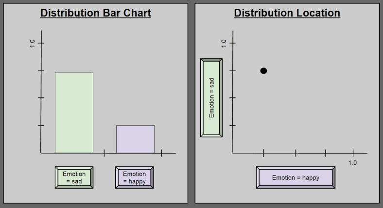
Consider a new variable, Emotion2 = { happy, sad }. Suppose we use this variable to describe a person undergoing a major depression. At any one time, such a person may have a 25% chance of being happy, and a 75% chance of being sad. This state of affairs can be described in two ways:

categorical_simplex_barchart_vs_loc

Pause here until you can explain to yourself why these diagrams are equivalent.

A Modest Explanation Of All Emotion

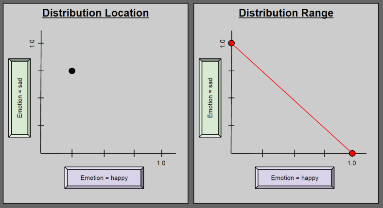
We have seen how a particular configuration of Emotioncan accurately characterize a depressed person. But Emotionis intended to describe all possible human emotion. Can it take on any value in this two-dimensional space? No: to describe a human being as P(happy) = 1.5; P(sad) = -0.1 is nonsensical. So what values besides (0.25, 0.75) are possible for Emotion2?

categorical_simplex_loc_vs_range

The above range diagram (right side) answers our question: any instance of Emotion2 must reside along the red line. Take a second to convince yourself of this. It sometimes helps to think about the endpoints (0.0, 1.0) and (1.0, 0.0).

Bar Charts Are Hyperlocations

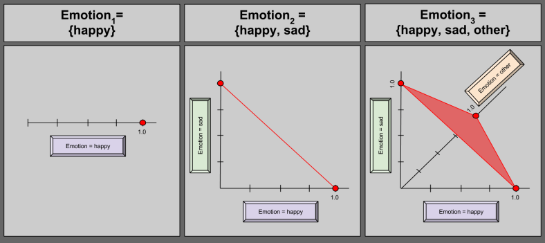
Perhaps you are not enthralled with the descriptive power of Emotion2. Perhaps you subscribe to the heresy that certain human experiences cannot be usefully described as either happy or sad. Let us expand our model to catch these “corner cases”, and define Emotion3 = { happy, sad, other }.

Can we identify a distribution range of this new variable? Of course!

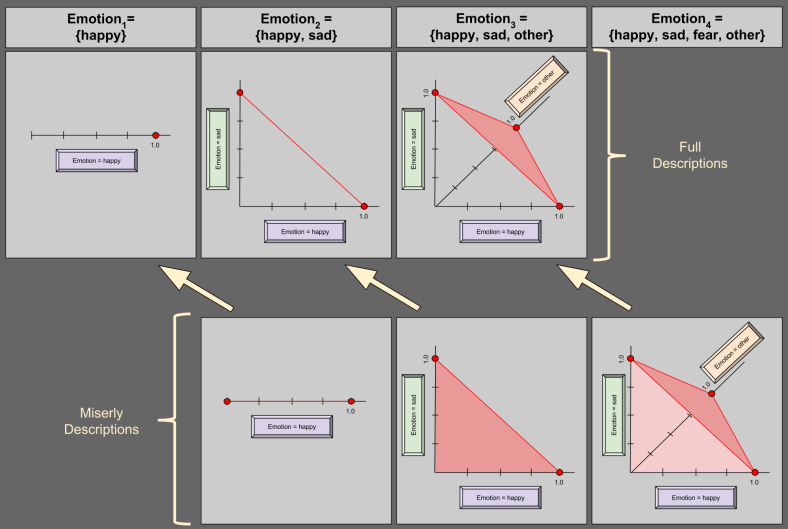
Probability Simplex- 1 vs 2 vs. 3 variables (1)

Take a moment to convince yourself that Emotion3 may never contain any point outside the shaded red area.

Alright, so we have a fairly pleasing geometric picture of a discrete random variables with domains up to size 3. But what happens when we mature our model again? Imagine expanding our random variable to encapsulate the six universal emotions.

Could you draw a bar chart for an arbitrary Emotion6?

Of course you could; you’d simply need to add four more bars to the first diagram of this post.

Now, what about location in space?

Drawing in 6-D is hard. 🙂

Here is the paradox: a simple bar chart corresponds with a cognitively intractable point in 6-dimensional space. I hope you never look at bar charts the same way!

An aside that, despite the constant three being sloppily hardcoded into our mental software, it turns out that reasoning about hyperlocations – points in N-dimensional space – is an important conceptual tool. If I ever get around to summarizing Drescher’s Good and Real, you’ll see hyperlocations used to establish an intuitive guide to quantum mechanics!

Miserly Description

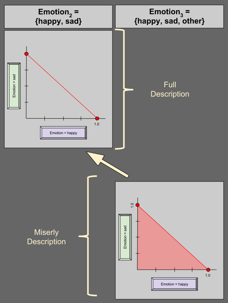
But do we really need 6-dimensional space to describe a domain of size 6? Perhaps surprisingly, we do not. Consider the case of Emotion3 = {happy, sad, other} again. Suppose I give you P(happy) = 0.5; P(sad) = 0.2. Do you really need me to tell you the P(other) = 0.3?

You could figure this out on your own, because the remaining 30% has to come from somewhere (0.3 = 1.0 – 0.5 – 0.2).

Given this fact that a variable has a 100% chance of being something (aka unitarity), we can describe a 4-variable in 3 dimensions:

Categorical Simplex- normal vs miserly description example

In the bottom-right of the diagram, we see an illustration of miserly description. Suppose we are given (0.25, 0.25) for happy and sad, respectively. P(other) must then be valued at 0.5, and (0.25, 0.25) is thus a valid distribution – this is confirmed by its residence in the shaded region above. Suppose I give you any point on the dark red edge of the region (e.g., (1.0, 0.0)); what value for P(other) must you expect? Zero.

This generalizes: unitarity allows us to describe an N-variable in N-1 dimensions. Here are two more examples:

Categorical Simplex- normal vs miserly descriptions

Notice the geometric similarities between the two descriptive styles, denoted by the yellow arrows.

The Hypervolume Of Probability

Consider the bottom row of our last figure (miserly descriptions). These geometric objects look similar: a triangle is not very different from a tetrahedron. What happens when we again move into a higher-dimensional space? Well, it turns out that there’s a name for this shape: a simplex is a generalization of a triangle into arbitrary dimensions. Personally, I would have preferred the term “hyperpyramid”, but I suppose the book of history is shut on this topic. 😛

We have thus arrived at an important result. The probability distribution associated with a discrete random variable can be represented as a simplex.

A Link To Convexity

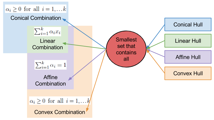
I want you to recall my discussion on convex combinations.

Convex Hulls

A convex combination should smell a lot like a probability distribution. Consider the axioms of Kolmogorov’s probability theory:

  1. The probability of an event is a non-negative real number.
  2. The probability that some event in the entire sample space will occur is 1.0
  3. The probability of the intersection of several events is equal to the sum of their individual probabilities.

If you compare these axioms to the maths of the above combinations, and squint a little, you’ll begin to hypothesize similarities. 🙂

It turns out simplices form a bridge between convex hulls and probability distributions, because a simplex simply is a convex hull.

Takeaways

  • Discrete random variables can refer to domains with more than two events.
  • As a description, a bar chart is interchangeable with a hyperlocation.
  • The range of possible probability distributions is relatively easy to characterize
  • We can describe one fewer dimension of a distribution by leveraging the fact of unitarity.
  • Such “miserly descriptions” reveal that all possible probability distributions of a categorical random variable is a generalized triangle (a simplex).
  • This geometric result reveals a deep connection between the foundations of probability theory and convex analysis.

[Sequence] Causal Inference

Background Material

Rubin’s Causal Framework:

Pearl’s Framework:

Applications

External Resources

Semirings As Algorithmic Parameters

Part Of: Graphical Models and Algebra sequence

In this, my final project in EE512A, I discuss how abstract algebra can be applied fruitfully in inference problems.

This project leverages some of the research conducted in the following posts:

My four page writeup is available here. My summary video is available here:

Intellectual History (2011-2014)

An incomplete list, which only covers books and courses (not articles) I have fully consumed (vs. started)

2011

  • Your Inner Fish [Shubin (2008)]
  • Structure Of Scientific Revolutions [Kuhn]
  • Open Society and its Enemies [Popper]
  • Who Wrote The Bible? [Friedman]
  • Don’t Sleep There Are Snakes [Everett]
  • Cows, Pigs, Wars, Witches [Harris]
  • A History Of God [Armstrong]
  • Witchcraft, Oracles, Magic among Azande [Evans-Pritchard]
  • Why Zebras Don’t Get Ulcers [Sapolsky]
  • The Trouble With Testosterone [Sapolsky]
  • The Myth Of Sisyphus [Camus]
  • Dialogues Concerning Natural Religion [Hume]
  • [Lecture Series] Philosophy Of Death [Kagan]
  • [Lecture Series] Human Behavioral Biology [Sapolsky]
  • [Lecture Series] Yale: New Testament Literature & History [Martin]
  • [Lecture Series] Philosophy Of Science [Kasser]
  • [MOOC] Intro To AI

2012

  • Influence [Cialdini]
  • The Origin Of Consciousness and Breakdown of the Bicameral Mind [Jaynes]
  • Hero With A Thousand Faces [Campbell]
  • Beyond Good and Evil [Nietzsche]
  • Genealogy Of Morals [Nietzsche]
  • Lost Christianities [Ehrman]
  • The Modularity Of Mind [Fodor]
  • Five Dialogues: Euthyphro, Apology, Crito, Meno, Phaedo [Plato]
  • The Mind’s I [Dennett]
  • The Protestant Ethic and the Spirit Of Capitalism  [Weber]
  • Interpretation Of Dreams [Freud]
  • Good and Real [Drescher]
  • In Two Minds [Evans, Frankish]
  • Thinking Fast and Slow [Kahneman (2011)]
  • Working Memory: Thought and Action [Baddeley]
  • Philosophy Of Mind [Jaworski]
  • [Lecture Series] Brain Structure And Its Origins [Schneider]
  • [Lecture Series] Justice [Sandel]
  • [MOOC] Machine Learning [Ng]
  • [MOOC] Health Policy & The ACA
  • [MOOC] Networked Life

2013

  • Evolutionary Physchology 4th edition [Buss (2011)]
  • Vision [Marr (1982)]
  • The Visual Brain in Action [Milner, Goodale (2006)]
  • Foundations Of Neuroeconomic Analysis [Glimcher]
  • Flow: The Psychology Of Optimal Experience [Csikszentmihalyi]
  • Architecture Of Mind [Carruthers (2006)]
  • [UW Course] CSEP524 Parallel Computation [Chamberlain]
  • [UW Course] CSEP514 Natural Language Processing [Zettlemoyer]
  • [UW Course] CSEP576 Computer Vision [Farhadi]

2014

  • The Conservative Mind [Kirk]
  • Guns, Gems, and Steel [Diamond]
  • Semiotics For Beginners [Chandler]
  • Rationality and the Reflective Mind [Stanovitch]
  • The Robot’s Rebellion [Stanovitch]
  • The Righteous Mind [Haidt]
  • The Selfish Gene [Dawkins]
  • The Better Angels Of Our Nature [Pinker]
  • The Illusion Of Conscious Will [Wegner (2003)]
  • [UW Course] CSEP590 Molecular and Neural Computation [Seelig]
  • [UW Course] CSEP573 Artificial Intelligence [Farhadi]
  • [UW Course] EE512A Advanced Inference In Graphical Models [Bilmes]

The Semiring Lifting Trick

Part Of: [Advanced Inference In Graphical Models] sequence

Table Of Contents

  • Motivations
  • Nested First-Order Semirings
  • Recursive Operator Resolution
  • Future Directions
  • Conclusion

Motivations

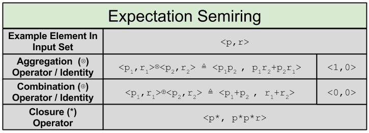
In 2002, Jason Eisner published Parameter Estimation for Probabilistic Finite-State Transducers in which he announced the discovery of the expectation semiring. This algebraic template is effectively used in the context of inferring parameters in a finite-state transducer (FST) model in the light of training data. The expectation semiring has the following structure:

Eisner- First-Order Semiring

Why are expectation semirings cool?

The weights from the expectation semiring are used to compute first-order statistics (e.g., the expected hypothesis length, or feature counts).

In 2009, Zhifei Li and Jason Eisner jointsly published First- and Second-Order Expectation Semirings with Applications to Minimum-Risk Training on Translation Forests.  This paper extended the previous paper by moving from a FST model to a hypergraph model, but also presented the variance semiring

Eisner- Second-Order Semiring

Why are variance semirings cool?

The variance semiring computes second-order statistics (e.g., the variance of the hypothesis length or the gradient of entropy). The variance semiring is thus essential for many interesting training paradigms such as minimum risk, deterministic annealing, active learning, and semi-supervised learning.

Our question today:

Is there a connection between these semirings?

Nested First-Order Semirings

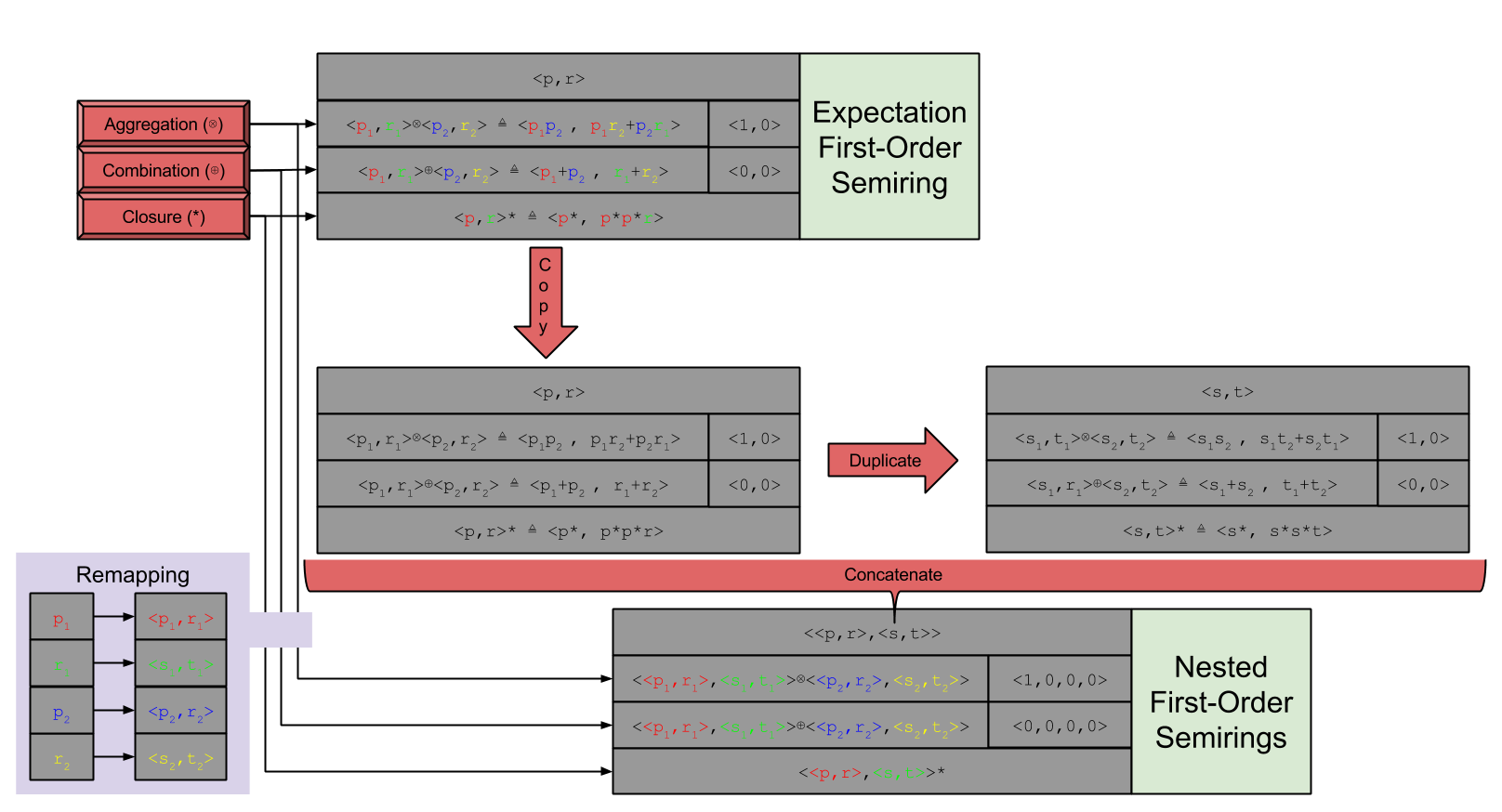
To create a nested first-order ring, simply duplicate the original, and concatenate the two semirings together:

Eisner- Lifting Trick Part One

Notice the remapping section, where we map each nested pair to a single argument to the semiring operators. This is also captured in my use of color.

Recursive Operator Resolution

Once you have these re-mapped the nested semiring, you must simply apply the original operators repeatedly. It is worth noting that the original semiring interpreted ⊗ in terms of multiplication, so we must recast multiplication back to ⊗ as many times as we recurse into the operator chain.

Eisner- Lifting Trick Part Two (2)

As you can see, after our algebra machine finishes, the second-order semiring is synonymous with our previously-discovered result of the variance semiring.

Future Directions

So we possess a mechanism by which we can transform the expectation semiring into the variance semiring. Here’s a “before & after”:

Eisner- Lifting Trick Summary (1)

So what? Is this all just a post-hoc rationalization, an attempt to explain why the variance semiring is useful after the fact?

I believe not. Eisner is not the only theoretician using semirings, but he is the only one (to my knowledge) to propose second-order semirings.

How might other researchers go about discovering new second-order semirings? Well, one immediate first step would be to apply the lifting technique to known-viable semirings, and see what happens! 🙂

Conclusion

Let me conclude with my list of open questions:

  • Do any viable semirings known today in fact support the lifting trick?
  • Quarternions were derived from complex numbers, from (a+bi) to [(a+bi)+(c+di)j]. What explains this analogue?
  • Could third-order semirings be productive?

Injection, Surjection, Bijection

Part Of: Algebra sequence
Content Summary: 600 words, 6 min read

Function As Operator

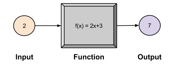
A function can be conceived as a machine that converts input into output. For example:

Bijection- Function As Operator

Something cool noticed by geometers of long ago:

If I feed the above function ALL POSSIBLE NUMBERS, I get a line!

Function As Map

We can also view functions as maps, taking an input value & returning its corresponding output item.

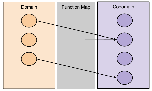
Let domain represent the set of all numbers that an input could be. Let codomain represent the set of all numbers that an output could be.  For example:

bijection-function-as-map-1

Counting Edges

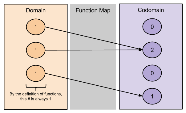
How might we classify different functions? One obvious thing to do is to count the number of edges entering or leaving a node:

bijection-counting-codomain-popularity

The definition of function is such that every input element maps to one and only one output element.  (This is why vertical lines are difficult to achieve in geometry). So the domain counts are relatively predictable.

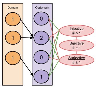
The codomain numbers, on the other hand, are fairly interesting. We can distinguish popular outputs as those with more than one entry, and unpopular outputs as those with no entries.

Injection & Surjection (& Bijection)

Suppose we want a way to refer to function maps that produce no popular outputs, whose codomain elements have at most one element. Call such functions injective functions.

Suppose we want a way to refer to function maps with no unpopular outputs, whose codomain elements have at least one element. Call such functions surjective functions.

If neither popular nor unpopular outputs exist — if all outputs are “normal” 🙂 — we may call such functions bijective functions.

The above example is neither injective nor surjective:

bijection-all-three-properties

Examples of all four outcomes:

bijection-all-four-outcomes

Cardinality vs. Bijection

Consider the bottom-left example. Note that its domain is smaller than its codomain (3 < 4). If I let you rearrange the arrows any which way, could you manufacture surjection? Take a minute to convince yourself that you cannot. Do you see why there will always be at least one unpopular output? Consider the top-right example. Note that its domain is larger than its codomain (4 > 3). If I allow you to rearrange the arrows any which way, could you manufacture injection?

Take a minute to convince yourself that you cannot. Do you see why there will always be at least one popular output?

The argument you must use to convince yourself of the above is an analogue to the pigeonhole principle.

More generally, we find that:

Bijection- Domain Cardinality Implications (1)

You can also use the above properties to “work backwards”: for example, if two sets provide at least one bijection, their relative sizes (cardinalities) must be equal.

Generalizing To Morphisms

When in doubt, zoom out! Time to fall in love with category theory. 🙂

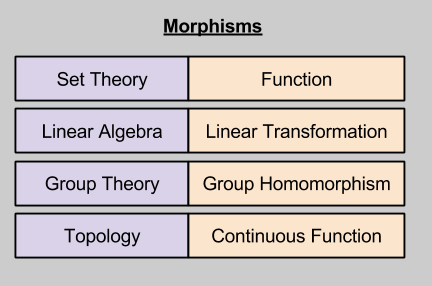
Functions that are grounded in set theory. But other types of structure-preserving maps have been studied:

Bijection- Generalizing Functions (1)

Injection/Surjection/Bijection were named in the context of functions. Wouldn’t it be nice to have names any morphism that satisfies such properties? Well, you’re in luck!

Bijection- Extending To Homomorphism (2)

Recall that bijection (isomorphism) isn’t itself a unique property; rather, it is the union of the other two properties.

It turns out that another interesting property to read out of maps is endomorphism: a map of an algebraic structure to itself. That makes three interesting properties. Let us explore how the sets of homomorphisms (a homomorphism is an general instance of a morphism, kind of like the instantiation of an abstract class in computer science) relate to each other:

Bijection- Set Relations Including Endomorphism

Decoding the above figure:

  • Hom set of homomorphisms
  • End → set of endomorphisms
  • Mon set of monomorphisms (i.e., injective morphisms)
  • Epi → set of epimorphisms (i.e., surjective morphisms)
  • Iso → set of isomorphisms (i.e., bijective morphisms)
  • Aut → set of automorphisms (i.e., bijective morphisms that also satisfy the endomorphic property)
  • →  contain only homomorphisms from some infinite structures to themselves.