
Part Of: Demystifying Sociality sequence
Followup To: The Three Spheres of Culture
Content Summary: 1700 words, 17 min read
A Theory of Relationship Dynamics
How can we make sense of social life? Let’s start by considering a simple cup of coffee.
- In my own house, I can just help myself to as much as I want, sharing with others in the framework of “what’s mine is yours.”
- Or my friend can get me a cup of coffee in return for the one I got for him yesterday, so we take turns or match small favors for each other.
- At Starbucks, I buy my coffee, using price and value as the framework.
- To my children, however, none of these principles apply. To them, coffee is something that only “big people” are allowed to drink: It is a privilege that goes with social rank.
What is true of a humble cup of coffee is true of the moral dilemmas surrounding major policy questions such as organ donation. Decisions have to be made, and there are again four fundamental ways to make them:
- Should we hold a lottery, giving each person an equal chance?
- Should we somehow rank the social importance of potential recipients?
- Should we sell organs to the highest bidder?
- Or should we expect everyone in a local community to give freely, offering a kidney to anyone group member in need?
(The above excerpt is from [FE] )
Relational Models Theory (RMT) proposes that these four social categories are exhaustive and culturally universal. Human interactions are complex, and typically use more than one of the above processes. But every relationship, in every culture, seems to be some combination of the following:
- In Communal Sharing (Communality), people are viewed as equals oriented around some particular identity. This can include being in love, sports fans, and co-religionists.
- In Authority Ranking (Dominance), people are situated in a hierarchy where superiors are deferred to, respected, and in some cases obeyed.
- In Equality Matching (Reciprocity), people are interested in restoring balance, turn-taking, and making sure everyone is treated fairly.
- In Market Pricing (Exchange), relationships are governed by quantitative, utilitarian concerns such as prices, exchanges, or cost-benefit analyses.
We can use relational models to explain a wide swathe of social phenomena:
- Some examples of norm violation are in fact category errors. For example, we would interpret a situation such as the price of our meal is two hours on dishwasher duty as a conflation of Market Pricing vs. Equality Matching.
- Some (but not all) examples of taboo trade-offs are in fact category errors. The Finite Price of Human Life thesis feels counterintuitive because it pits our Market Pricing versus the sacred values held by Communality.
- Humans often use indirect speech acts to reconcile relationship types with semantic content.Rather than saying e.g., “pick me up after work”, we often say things like, “If you would pick me up after work, that would be awesome”. While more verbose, the latter expression feels more polite because it is couched in a Communality frame, rather than signaling Dominance.
In addition to its explanatory reach, multiple strands of evidence come together in support of Relational Model theory:
- Factor analysis. If you ask people to describe their relationships, you can see whether your theory predicts statistical patterns in their responses. When RMT was compared with other taxonomies (and there are a lot of them), RMT starkly outperforms its competitors.
- Ethnographies. RMT was invented by anthropologist Alan Fiske to capture regularities he saw across different cultures. For example, he found examples of marriage treated as Dominance, as Market Pricing, etc – but never a fifth type. A number of cross-cultural studies indicate that the four relational models constitute a human universal.
- Social errors. When people misremember a person’s name, it tends to be a person with whom they share the same relationship type. For example, if you flub the name of your boss, you are more likely to say the name of someone else in a position of authority over you.
- Brain studies. In the cortex, the default mode network is universally acknowledged to perform social processing. But within this specialized region, different subregions are activated when processing e.g., Communality vs Reciprocity relationships.
The Relational Sphere Hypothesis
Human societies can be conceived as operating in three spheres: markets, governments, and communities. The Cultural Sphere Hypothesis holds this trichotomy to be fundamental, and exhaustive of social space.
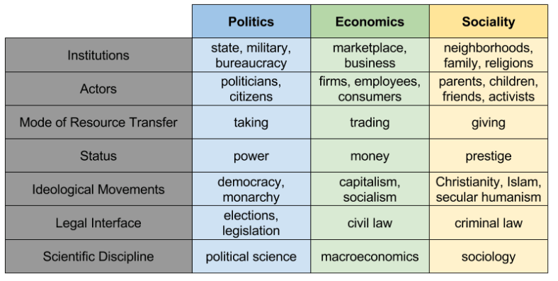
There seems to be a relationship between the cultural spheres and relation models. But there are three spheres vs four models. What gives?
Things become more clear when we remember that market- based economies were invented during the Neolithic Revolution, with the dawn of agriculture. Before this inflection point in history, transactions took place with gift economies.
This suggests that the Market Pricing relational model is evolutionarily recent: before the invention of agriculture, it simply did not exist.
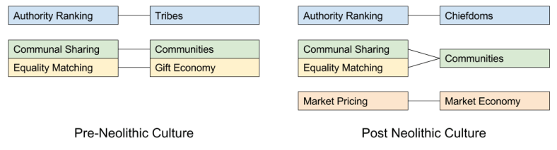
I call this particular mapping from relational models to cultural spheres the Relational Sphere Hypothesis (RSH). It is an intertheoretic reduction: it purports to be a significant join point between micro- and macro-sociality.
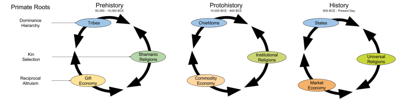
RSH predicts that three out of four relational models can be traced back to the birthplace of Homo Sapiens. Thus, we should expect predecessors for these relationship categories in primate societies! And we find precisely that:
- Dominance models are expressed in the dominance hierarchy (where physical dominance slowly gave way to symbolic dominance).
- Communality models are expressed in kin selection (where attachment to and care for relatives was slowly extended towards e.g. close friends).
- Reciprocity models are expressed in reciprocal altruism (where increasingly large delays between favor-transactions became possible).
I have argued elsewhere that the dual-process models so popular in today’s moral psychology can be captured in the interactions between (cortical) propriety frames and (subcortical) social intuitions. These two systems comprise the building blocks of sociality. RSH dovetails nicely with this dual process account, as it perceives categories within these systems, each with its own distinctive logic:
With the exception of Sanctity, these subconscious social intuitions arguably exist in primates. For example, here is evidence that rhesus monkeys have strong intuitions about Fairness:
A New Kind of Social Network
The Relational Sphere Hypothesis can be further illustrated by social networks: graphs where nodes are individuals, and edges are relationships. These kinds of models are very common across many disciplines that study aggregate social phenomena; for example evolutionary game theorists. A social network may look something like this:
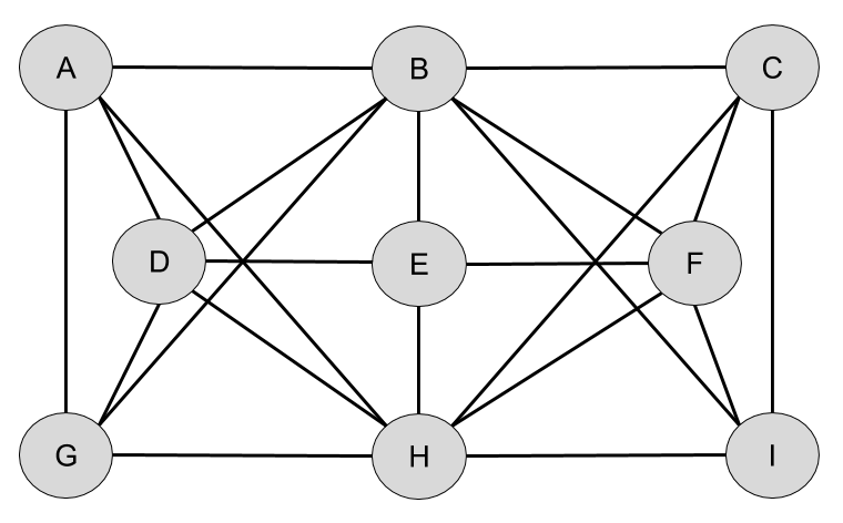
But relationships inhabit different categories. We can express this fact by coloring edges according to their relational model:
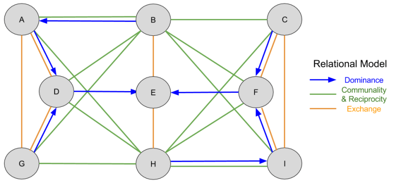
Note that some nodes (e.g. A and B) are connected by more than one color. This signifies that the relationship between A and B features both Communality and Dominance.
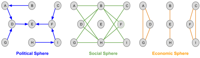
From this more complete picture of human relationships, we can derive our cultural spheres by examining the (mono-color) subgraphs:
Sphere Evolution & Competition
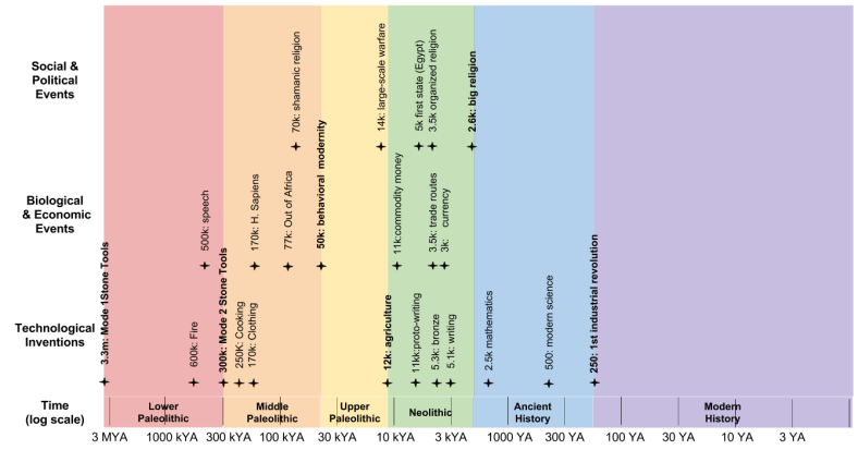
Political, social, and economic institutions have dramatically changed across the course of human history. As we saw in Deep History of Humanity, the evolution of our species can be usefully divided into three time periods:
The Sphere Competition Conjecture comprises a set of informal intuitions that relational models “competes for our attention”: gains in one sphere are often accompanied by losses in another.
Let me illustrate this conjecture with examples. 🙂
Social vs Economic spheres
- The religious instinct is etched deeply into the hominid mind, and evidence for shamanic animism dates back to the advent of behavioral modernity. Modern religion is located squarely within the Social sphere. But what caused its institutionalization, the invention of the full-time religious specialist: the priest? Religious institutions were founded during the transition from gift economy to market economies. For the first time in history, material wealth mattered more in transactions than interpersonal reputation. With the Social sphere threatening to collapse, perhaps it is not a coincidence that it was at this moment in history that religion became more explicitly social.
- Some existential philosophers argue that the industrial revolution, with its obscenely large increase in Economic productivity, has correlated with a weakening of Social values, as witnessed empirically by the rise of materialism. Perhaps the malaise and cynicism of postmodernity can be explained by the weakening of the ties of community.
- The custom of tipping can be conceived as an organ of Sociality, that feels misplaced in today’s Market-oriented economy. This institution shows no signs of abating (for example, Uber recently rescinded its no-tipping policy). Perhaps the reason this Social technology persists, while others have disintegrated, is because tipping solves the principal agent problem: customer service is otherwise not factored into the price, because that information is not easily available to management.
- Product boycotts are another example of Social outrage affecting Economic markets.
Social vs Political.
- Another important event in the history of religion is the transition to universal religions: where the concerns of the gods and the consequences of moral violations were imbued with an aura of the eternal. Anthropological evidence clearly suggests that universal religions succeeded because they facilitated larger group sizes.
- Corruption is often treated as a political problem, but in fact bribery and collusion both require high amounts of social capital.
- In American history, political partisanship has been most severe in the 1880s, and at present. Both then and now are periods of an intense drought of social capital. Further, participation in voting strongly correlates with vibrant community and civic life. We might conjecture that weaker communities are more vulnerable to partisanship infighting. This conjecture is aligned with the oft-cited observation that partisanship tends to correlate with moderates abandoning the political arena.
Economic vs Political.
- Capitalist Peace Theory formalizes the observed inverse relationship between free trade and international conflict. On this hypothesis, one of the strongest predictors of war is resource acquisition, and the risk-benefit calculus changes (improves) substantially with the removal of tariffs.
Economic vs Political vs Social.
- The Size of Nations Hypothesis is the idea that the size of nation (Political) is driven by two competing factors: larger nations are able to produce public goods more efficiently (Economic), but conversely their populations are more heterogenous and thereby less cohesive (Socially).
Some of the phenomena described above have been extensively studied by social scientists. However, to my knowledge, no extant models robustly capture the doctrine of relational model theory. Perhaps the next generation of formal models will do better.
Recommended Resources
- [FE] Fiske, Ehrenhalt. Basic Relationships. Accessible here (first link)
- [Has04] Haslam (2004). Relational Models Theory: A Contemporary Overview
- [Wick09] Wick’s (2009). A Model of Dynamic Balance among the Three Spheres of Society.
- Pinker’s take on Relational Models Theory, Animated
- RMT Research Bibliography


 and
and  . We will denote
  as
as  . We will use this notation instead of the more common
  . Both represent the idea “apply
  .
. 

 isn’t even a
  to the underlying set exacerbates the problem: then both
  and
and  .
.
 denotes composition over a set of all bijections (permutations) over some set of
  objects. The symmetric group is then of order
  .
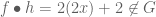
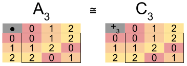
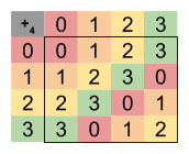
. is the set of all permutations over a 3-element set. It is of order
  .
. . The top row represents the original elements
  , the bottom represents where each element has been relocated
  .
. 
 has two permutations with 3-cycles: can you find them?
 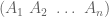 , pronounced “
 goes to
  goes to …”.
 .
. and
and  , take each element
  and follow its arrows until you find the set of disjoint cycles. More formally, compose these functions
  .
.  .
.
 .
. 
 ) can be omitted: their inclusion does not affect algorithm results.
 . Contrast this with composition, which does not commute
  .
.
 ? It is isomorphic to
 and
and  resemble rotations/cycles;
  ,
,  , and
, and  perform reflections/flips.
 has three transpositions
  ,
,  , and
, and  .
. . In fact, we can lay claim to an even stronger fact:
 .
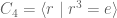
. , we can generate our “dihedral-looking” Cayley graph by selecting generators
  and
and  .
. .
. .
. .
. 
 means a green arrow
  .
. , because arrows in the latter are monochrome and unidirectional.
 ,
,  . And we can confirm by inspection that, in fact,
  etc.
etc.
 . These have 2, 4, and 8 permutations, respectively.
  . These have 3, 5, and 9 permutations, respectively.
 are even permutations.
 of odd permutations.
 . Just as
  ,
,  elements.
  in more detail. Does it remind you of anything?
 ..!
..!
 . Is it also true that e.g.,
  and
and  ?
? and
and  . Only
  , these sets are not even potentially isomorphic. For example:
 .
. .
. .
.
 .
.
 . However, for larger
  ). Are finite groups possible?
 . Is it a group? No, it isn’t even a magma:
  ! Is there a different operation that would produce closure?
  , on
, on  . For example,
  .
.
 .
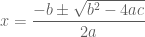
. is an
is an  . Its solutions, or roots, is the set
  . This set is called the fourth roots of unity.
 ? In the following table, recall that
  , thus
  .
.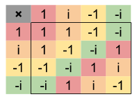
 . Let’s compare the function maps of our two groups:
 . Let
. Let .
.
 . Inspection reveals that this, too, is isomorphic to
  !
! , there exists some generator
  , where r is any generator.
 .
.
 . But you can also recreate them by
  .
.  , or multiplying by
  . Only
  fails to be a generator.
  rotation, and counterclockwise
  .
. .
. .
.  ? All non-identity elements:
  .
.  .
. configurations. It would take a long time just writing down such a group. But it has only six generators (one for a
 .
. .
. suffix is often left implicit from presentations (e.g.,
  ) for the sake of concision.
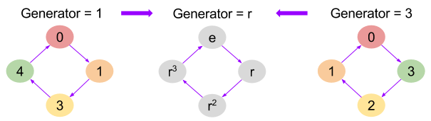
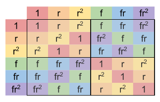
 . Let us consider the “triangle group”
  rotation
  and a horizontal flip
  . Similarly, two flips returns to the identity
  . Is there some combination of rotations
 .
.
 .
.
 is not abelian: its multiplication table is not symmetric about the diagonal.
 table with a
  table. We will explore this intuition further, when we discuss quotients.
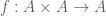
 is a mapping from the elements of one set to another. Further, i
 .
. .
. .
. , for any two integers. In fact there exist five such axioms:
 .
. .
. such that,
  .
. there exists an element
  such that
  .
. .
.
 . Multiplication too can be described with five axioms:
 .
. .
. .
. such that
  .
. .
.
 . Note that
  is just shorthand for the more formal
  . Note that the operation symbol
  is just a name: we could just as easily rename the above function to be
  , as long as the underlying mapping doesn’t change.
 ) has arity-1. A finitary operation has arity-n.
 .
. .
. such that,
  .
. there exists an element
  such that
  .
. .
.
 ) and commutativity (
 ). Likewise, the natural numbers under subtraction are not even a magma:
  .
.  matrices under matrix multiplication?
 ![I = [ \begin{smallmatrix}1 & 0\\0 & 1\end{smallmatrix}]](https://s0.wp.com/latex.php?latex=I+%3D+%5B+%5Cbegin%7Bsmallmatrix%7D1+%26+0%5C%5C0+%26+1%5Cend%7Bsmallmatrix%7D%5D&bg=ffffff&fg=555555&s=0&c=20201002) .
. 
 and
and  When do we call these lines parallel? When their slopes are equal
  . We can gain insight into the situation by mapping
  and
and  form the horizontal and vertical axes respectively.
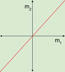
 and
and  being placed in an
  . We denote their intersection as
  . Let us compare the dimensions of these three manifolds to the dimension of their overlap.
  as
as  respectively. Now our examples can be expressed as 4-tuples
  :
:


 ?
?  , that the two planes intersect at a point, you have noticed the pattern!
  . The overflow is defined as
 , the submanifolds do not intersect:
 , the intersection is non-empty
  , and
, and 

 vs.
vs.  vs.
vs.  vs.
vs.  vs.
vs.  vs.
vs.  :
: , then generically, a crossing is possible (at all times,
  , then generically, a crossing is not possible (at some time,
  is the following movement possible?
 . But Theorem 4 says that, if the ambient dimension is four, then the overflow is
  , so crossing is possible.
 and
and  represent the beginning and end positions as it travels throughout time
 ![t \in [0,1]](https://s0.wp.com/latex.php?latex=t+%5Cin+%5B0%2C1%5D&bg=ffffff&fg=555555&s=0&c=20201002) . If
. If  never has self-intersection at any time
  , we say
 : this is why it is called
  : we can unwind the trefoil knot in
  : simply lift the top-left string up.
  to
to  : you only need
 , knots self-intersect. In
 ; after all
  .
. :
:
 ). If we isotope along its surface using
  , is
, is  ? How about
  ?
? 
 . You just pull the circle left, along that surface of the torus.
 . You might suspect you can just pull the blue circle over the middle hole. But that would require leaving the surface
  (but
(but  ).
). represents the set of fruits which I prefer.
 can represent, among other things, the fingers on my left hand.
 .
. .
. and
and  expresses the very same set.
  . We will prefer to express sets with the latter, more compact, notation.
 is a perfectly valid two-element set, quite distinct from the three-element set
  .
. ) if A and B contain exactly the same elements.
 and
and  . Then,
  . Then,
  .
. . Otherwise, we write
  .
. . Then
  means “yellow is an element of the set of primary colors”.
 means “-1 is not an element of the natural numbers”.
 . The element
  : only the set
  is.
is. , its
, its  , is the number of elements in that set.
 .
. . Then
  . Note that cardinality only looks at “the outer layer”.
  is the set containing no elements.
  .
. .
. .
.  , where the | symbol is pronounced “such that”.
 . In words “let A be the set of integers X such that x is greater than zero and less than six.”
 .
. and let
  . Here
  and
and  bits of computer memory, each bit of which is uniquely identified with a 6-bit address. Suppose further that our memory has been allocated to data structures of varying size. To promote addressing efficiency, a computer can adopt the following strategy: assign shorter addresses to larger variables.
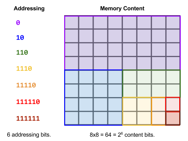
 , if every element of
  and
and  . Then
  . Then
  (C does not contain 9).
 ? Yes. For all
  is true.
 , if
, if  is the set of all subsets of
  . Then
  .
.
 , then
  .
. ) versus subset-of (
  ) relations. Consider again
  . But
. But  . The
. The  . But
. But  . The
. The  -algebras draw from the power set of natural numbers
  .
. is the set of all
  such that
  and
and  . Note that, unlike the elements in a set, the elements of an ordered pair cannot be reordered.
 and
and  . Then
  .
.
 . Thus,
  . This is because elements within ordered pairs cannot be rearranged.
 . In combinatorics, this observation generalizes to the multiplication principle.
 is a well-known example of a Cartesian product.
 , their Cartesian product is the set of all n-tuples.
 ,
,  and
and  . Now
. Now  .
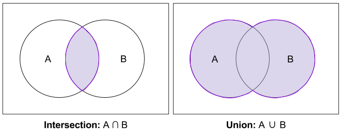
. , is the set of elements common to both sets.
 and
and  . Then
  .
. . Then
  .
. .
. is the set of all elements that are in
  .
. .
.
 . This
  is the set of elements in
  and
and  . Then
  and
and  .
. . Then
  and
and  .
. is the set of elements in
  .
.
 and let its universe be the set of complex numbers
  . It is true that
  .
. is the set of all elements of
  and
and 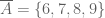 .
.

