Topology posts
Calculus posts
- An Introduction to Derivatives
- An Introduction to Integrals
Topology posts
Calculus posts
Part Of: Analysis sequence
Content Summary: 1000 words, 10 min read
Motivating Example
Can you draw three lines connecting A to A, B to B, and C to C? The catch: the lines must stay on the disc, and they cannot intersect.

Here are two attempts at a solution:

Both attempts fail. In the first, there is no way for the Bs and Cs to cross the A line. In the second, we have made more progress… but connecting C is impossible.
Does any solution exist? It is hard to see how…
Consider a simplified puzzle. Let’s swap the inner points B and C.
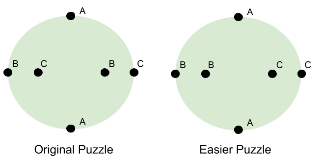
In the new puzzle, the solution is easy: just draw straight lines between the pairs!
To understand where this solution breaks down, let’s use continuous deformation (i.e., homeomorphism) to transform this easier puzzle back to the original. In other words, let’s swap point B towards C, while not dropping the “strings” of our solution lines:

Deformation has led us to the solution! Note what just happened: we solved an easy problem, and than “pulled” that solution to give us insight into a harder problem.
As we will see, the power of continuous deformation extends far beyond puzzle-solving. It resides at the heart of topology, one of mathematics’ most important disciplines.
Manifolds: Balls vs Surfaces
The subject of arithmetic is the number. Analogously, in topology, manifolds are our objects. We can distinguish two kinds of primitive manifold: balls and surfaces.
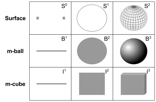
These categories generalize ideas from elementary school:
 is a line segment
 is a disc
 is a circle
 is a sphere
Note the difference between volumes and their surfaces. Do not confuse e.g., a disc with a circle. The boundary operation 

Note that surfaces are one dimension below their corresponding volume. For example, a disc resides on a plane, but a circle can be unrolled to fit within a line.
Importantly, an m-ball and an m-cube are considered equivalent! After all, they can be deformed into one another. This is the reason for the old joke:
A topologist cannot tell the difference between a coffee cup and a donut. Why? Because both objects are equivalent under homeomorphism:
If numbers are the objects of arithmetic, operations like multiplication act on these numbers. Topological operations include product, division, and connected sum. Let us address each in turn.
On Product
The product (x) operation takes two manifolds of dimension m and n, and returns a manifold of dimension m+n. A couple examples to whet your appetite:
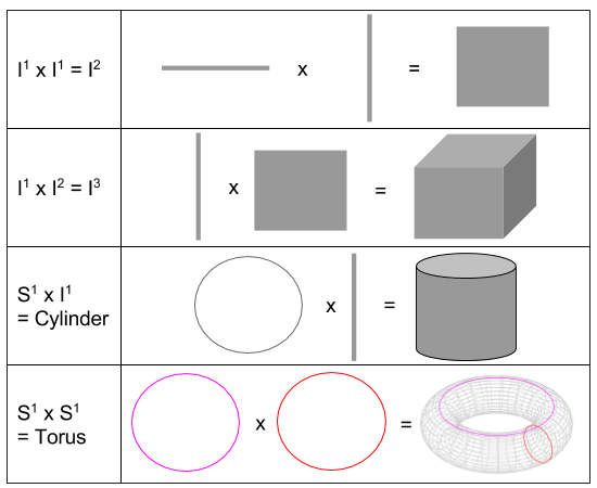
These formulae only show manifolds of small dimension. But the product operation can just as easily construct e.g. a 39-ball as follows:
How does product relate to our boundary operator? By the following formula:
This equation, deeply analogous to the product rule in calculus, becomes much more clear by inspection of an example:

On Division
Division ( / ) glues together the boundaries of a single manifold. For example, a torus can be created from the rectangle 
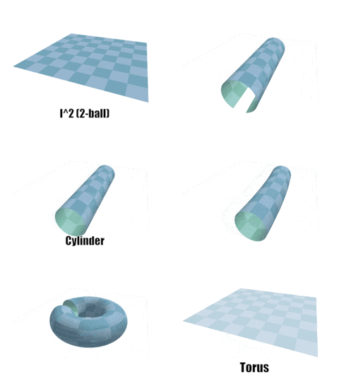
We will use arrows to specify which edges are to be identified. Arrows with the same color and shape must be glued together (in whatever order you see fit).
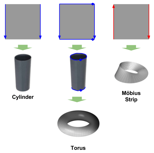
Alternatively, we can specify division algebraically. In the following equation, x=0 means “left side of cylinder” and x=1 means right side:
The Möbius strip is rather famous for being non-orientable: it neither has an inside nor an outside. As M.C. Escher once observed, an ant walking on its surface would have to travel two revolutions before returning to its original orientation.
More manifolds that can be created by division on
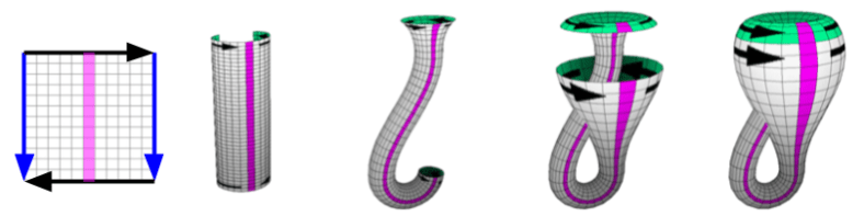
In our illustration, there is a circle boundary denoting the location of self-intersection. Topologically, however, the Klein bottle need not intersect itself. It is only immersion in 3-space that causes this paradox.
Our last example of 

The top portion becomes a Möbius strip; the bottom becomes a disc. We can deform a disc into a sphere with a hole in it. Normally, we would want to fill in this hole with another disc. However, we only have a Möbius strip available.
But Möbius strips are similar to discs, in that its boundary is a single loop. Because we can’t visualize this “Möbius disc” directly, I will represent it with a wheel-like symbol. Let us call this special disc by a new name: the cross cap.
The real projective plane, then, is a cross cap glued into the hole of a sphere. It is like a torus; except instead of a handle, it has an “anomaly” on its surface.

These then, are our five “fundamental examples” of division:

On Connected Sum
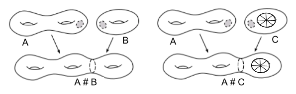
Division involves gluing together parts of a single manifold. Connected sum (#), also called surgery, involves gluing two m-dimensional manifolds together. To accomplish this, take both manifolds, remove an m-ball from each, and identify (glue together) the boundaries of the holes. In other words:
Let’s now see a couple examples. If we glue tori together, we can increase the number of holes in our manifold. If we attach a torus with a real projective plane, we acquire a manifold with holes and cross-cuts.
Takeaways
Related Materials
This post is based on Dr. Tadashi Tokeida’s excellent lecture series, Topology & Geometry. For more details, check it out!
Part Of: Language sequence
Followup To: An Introduction to Generative Syntax
Content Summary: 800 words, 8 min read
Explaining Substitution
Consider the sentence “I bought this big book of poems with the red cover”.

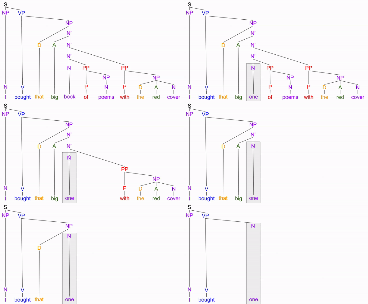
In everyday language, we often replace words and phrases with indexing words like “one”. Call this indexing replacement.The meaning of these words can be obtained from the context.
At first glance, indexing replacement seems to target a branch in the syntax tree. For example:
But there are several other substitutions don’t follow from branch replacement:
Perhaps our notion of noun phrases is too flat. Perhaps we need additional nodes to describe structure within the noun phrase. We will call these intermediate nodes N’, (where N → N’ → N’’ = NP):
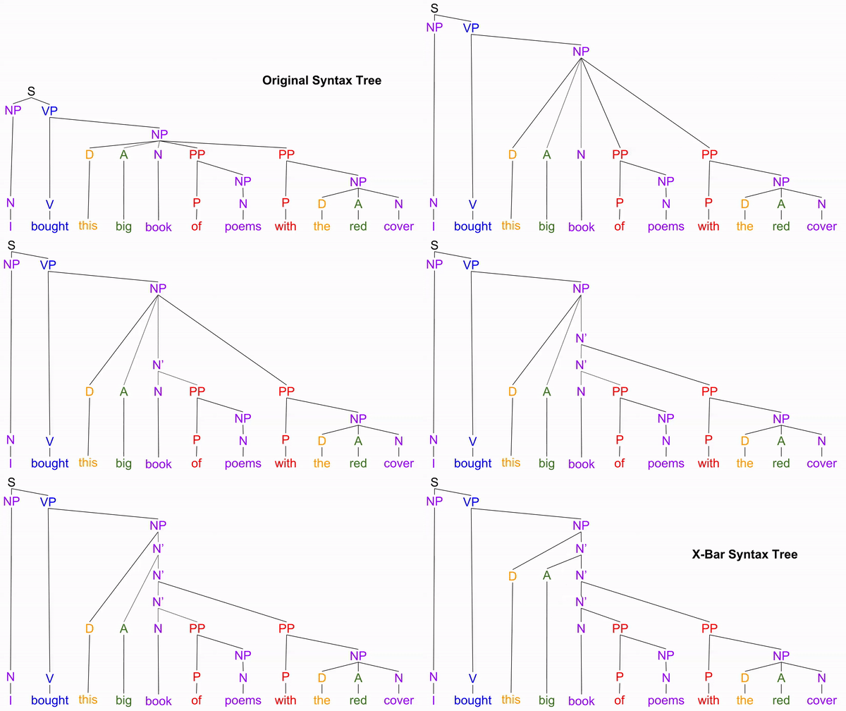
This new tree successfully predicts all substitution phenomena, by modeling “one” as replacing various “N-bar” nodes:
We can similarly introduce depth to our verb phrases (VPs), by using intermediate V’ (“V-bar”) nodes:
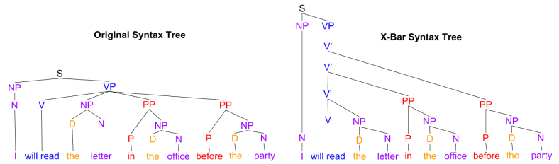
The X-Bar syntax tree provides a simple explanation of the “do so” substitution effects:
A General Theory of Phrases
We can revise our original NP and VP rules to reflect our intermediate N’ and V’ nodes:

What if noun and verb phrases are instantiations of a more general phrase structure? Just as group theory identifies overlap in the axioms of addition and subtraction, X-bar theory explores the similarity between NP and VP rules.
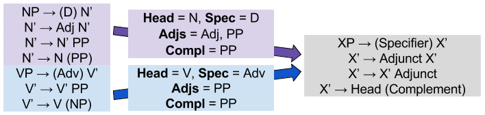
There are only four kinds of phrase constituents:
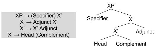
Adjuncts vs Complement
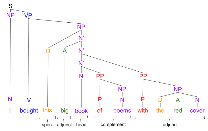
Given that adjuncts and complements both often inhabit prepositional phrases, it is perhaps surprising that they should behave differently. The distinction between adjuncts and complements explains why this should be the case. Let us look at four behavioral differences:
Difference #1. Adjuncts can be reordered freely.
Consider our example verb phrase:

This rule means that our two adjuncts can be shuffled, but the complement NP must retain its original position
Difference #2. Indexing replacement cannot strand the complement.
For example,
Consider another part of speech we have not yet considered: conjunction words like “and” and “or”.
Difference #3. Conjunction words bind adjuncts together, and complements together. But adjunct-complement bindings are non-grammatical.
Consider our example noun phrase:
Three examples to illustrate how conjunction works:
What X-Bar Theory Tells Us About Memory
Earlier, I introduced the distinction between episodic and semantic memory:
Concepts are learned by extracting commonalities from episodic memories. If you see enough metallic blocks moving around on four cylinders, you’ll eventually consolidate these objects into the CAR concept:
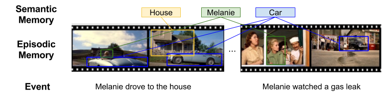
In philosophy, I suspect the concepts of necessity and contingency relate to semantic and episodic memory, respectively.
In linguistics, I suspect complements help locate concepts in semantic memory, whereas adjuncts assist episodic localization. In the sentence “I bought the book of poems with the red cover”, the complement helps us activate the concept POEM-BOOK, whereas the adjunct creates sense-predictions that locate it within our episodic memory.
Takeaways
Part Of: Language sequence
Content Summary: 900 words, 9 min read
Syntax vs Semantics
In language, we distinguish between syntax (structure) and semantics (meaning).
Compare the following:
Both sentences are nonsensical (a semantic transgression). But the first is grammatically correct, whereas the second is malformed.
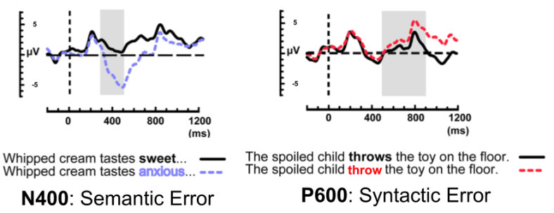
The brain responds differently to errors of syntax and semantics, as measured by an EEG machine. Semantic errors produce a negative voltage after 400 milliseconds (“N400”); syntactic errors produce a positive voltage after 600 milliseconds (“P600”):
Parts of Speech
To understand syntax more precisely, we must differentiate parts of speech. Consider the following categories:
Nouns and verbs correspond to perception- and action- representations, respectively. They are an expression of the perception-action cycle. But to study syntax, it helps to put aside semantic context, and explore how parts of speech relate to one another.
Phrases as Color Patterns
To understand syntax intuitively, start by adding color to sentences. Then try to find patterns of color unique to well-formed sentences.
Let’s get started!
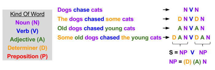
“Noun-like” groups of words appear on either side of the verb. Let noun phrase (NP) denote such a group. Optional parts of speech are indicated by the parentheses. Thus, our grammar contains the following rules:
These rules explain why the following sentences feel malformed:
But these rules don’t capture regularities in how verbs are expressed. Consider the following sentences:
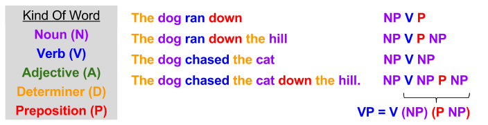
A verb phrase contains a verb, optionally followed by a noun, and/or a preposition.
This is better. Did you notice how we improved our sentence (S) rule? 🙂 Subject-only sentences (e.g. “She ran”) are now recognized as legal.
Prepositions are not limited to verb phrases, though. They also occur in noun phrases. Consider the following:

Prepositions are sometimes “attached to” a noun phrase. We express these as a prepositional phrase, which includes a preposition (e.g. “on”) and an optional noun phrase (e.g. “the table”).
Notice how we cleaned up the VP rule, and improved the NP rule.
Congratulations! You have discovered the rules of English. Of course, a perfectly complete grammar must include determiners (e.g., “yours”), conjunction (e.g., “and”), interjection (e.g., “wow!”). But these are fairly straightforward extensions to the above system.
These grammatical rules need not only interest English speakers. As we will see later, a variant of these rules appear in all known human languages. This remarkable finding is known as universal grammar. Language acquisition is not about reconstructing syntax rules from scratch. Rather, it is about learning the parameters by which your particular natural language (English, Chinese, Egyptian) varies from the universal script.
From Rules to Trees
Our four rules are polymorphic: they permit more than one kind of structure. Unique rule sets are easier to analyze, so let’s translate our rules into this format:
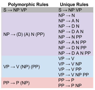
Importantly, we can conceive of these unique rules as directions to construct a tree. We can conceive of the sentence “Dogs chase cats” as:
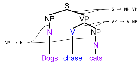
Sentences are trees. These trees are not merely used to verify whether grammatical correctness. They play a role in speech production: which transforms the language of thought (Mentalese) to natural language (e.g., English). For more on this, see my discussion of the Tripartite Mind.
How can (massively parallel) conscious thought be made into (painfully serial) speech utterances? With syntax! Simply take the concepts you desire to communicate, and construct a tree based on (a common set of) syntactical rules.
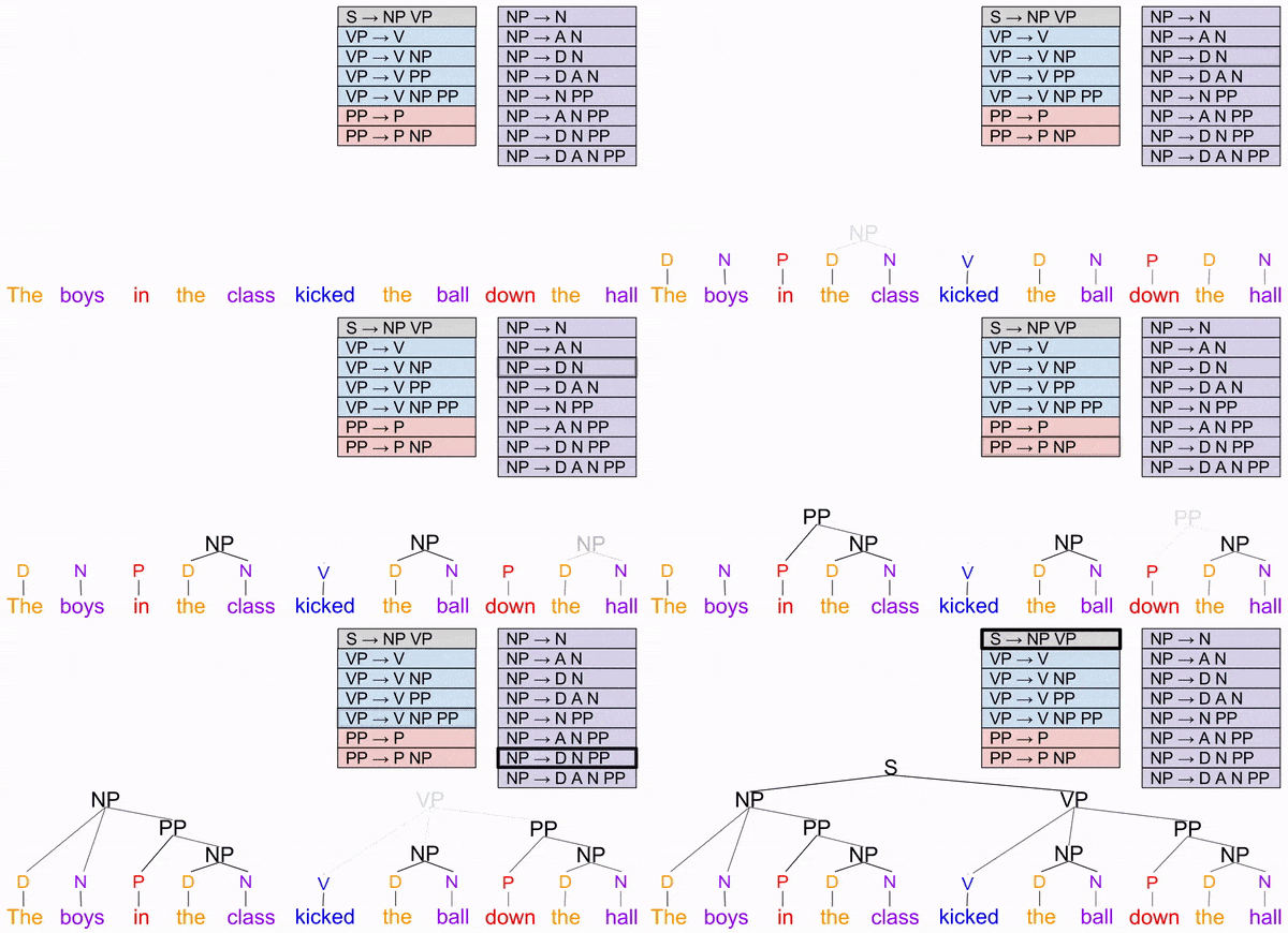
Tree construction provides much more clarity on the phenomena of wordplay (linguistic ambiguity). Consider the sentence “I shot a wolf in my pajamas”. Was the gun fired while you were wearing pajamas? Or was the wolf dressed in pajamas?
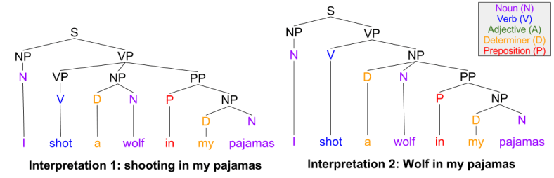
Both interpretations agree on parts of speech (colors). It is the higher-order structure that admits multiple choices. In practice, semantics constrain syntax: we tend to select the interpretation is feels the most intuitive.
The Sociology of Linguistics
The above presentation uses a simple grammar, for pedagogic reasons. I will at some point explain the popular X’ theory (pronounced “X bar”), which explores similarities between different phrase structures (e.g., NP vs PP). Indeed, there is a wide swathe of possible grammars that we will explore.
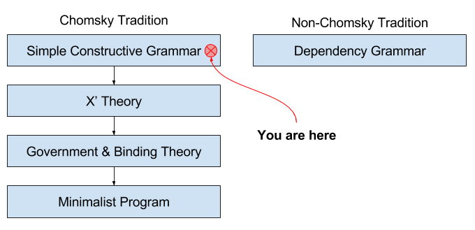
Generative grammar is part of the Symbolist tribe of machine learning. As such, this field has rich connections with algebra, production systems, and logic. For example, propositional logic was designed as the logic of sentences; predicate logic is the logic of phrases.
Other tribes besides the Symbolists care about language and grammar, of course. Natural Language Processing (NLP) and computational linguistics have been heavily influenced by the Bayesian tribe, and use probabilitic grammars (i.e., PCFGs).
More recently, the Connectionist tribe (and deep learning technologies) are taking a swing at producing language. In fact, I suspect neural network interpretability will only be achieved once a Connectionist account of language production has matured.
Takeaways
For more resources on syntax trees, I recommend this lecture, this website, and this Youtube channel.
Until next time.
Part Of: Logic sequence
Followup To: Natural Deduction
Content Summary: 600 words, 6 min read
Motivating Sequent Calculus
Last time, we labelled propositions in the language of verification.
Two of our connective rules (⊃I and ∨E) expanded our set of assumptions, which we could use at any later time. Logic acumen is invoking the right assumption at the right time.
In contrast to natural deduction, sequent calculus explicitly tracks the set of assumptions) as they vary across different branches of the proof tree.
We will use the turnstile to distinguish assumptions from conjecture: { assumptions } ⊢ { conjectures }
In natural deduction, progress in bidirectional: we are done when we found a connection between assumptions and conjecture. In sequent calculus, progress is unidirectional. Instead, we start with no assumptions, and finish when we have no conjectures left to demonstrate.

Both logical systems rely on two sets of five rules. They bear the following relationships:
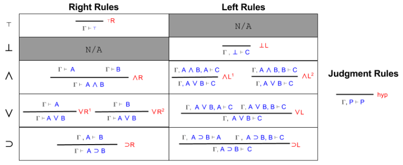
Right and Left rules
We here define capital gamma Γ to represent the context, or current set of assumptions.
Right rules simply preface Introduction rules with “Γ ⊢”. The exception ⊃R is instructive. There, A is added to the context, and our “target” conjecture shrinks to just B.

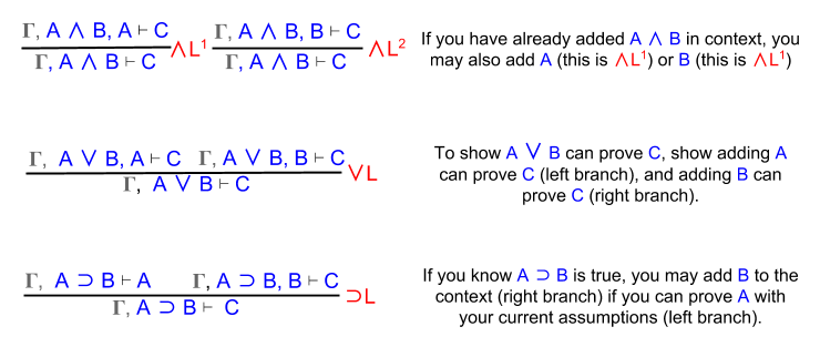
Left rules are less transparently related to Elimination. They are more easily understood by an English explanation:
The entire structure of sequent calculus, then, looks like this:
Enough theory! Let’s use sequent calculus to prove stuff.
Example 1: Implication
Show that (A ⊃ (B ⊃ C)) ⊃ ((A ⊃ B) ⊃ (B ⊃ C)).
Here, ⊃R serves us well:

We have parsed the jungle of connectives, and arrived at a clear goal. We need to prove C. How?
Recall what ⊃L means: “if you have assumed A ⊃ B, you may also assume B (right branch) if you can prove A with your current assumptions (left branch).
Let’s apply ⊃L to the A ⊃ B proposition sitting in our context. To save space, let us here define Γ with the following three elements: { A⊃(B⊃C), A⊃B, and A }.
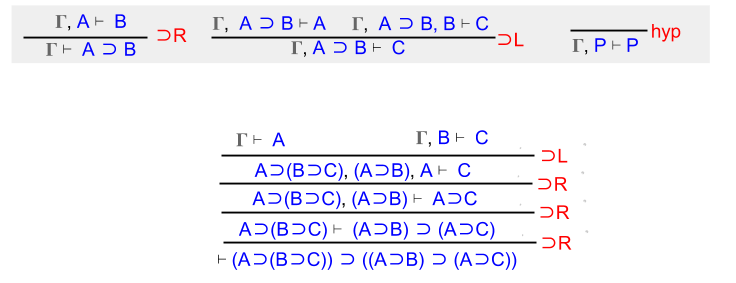
We can solve the left branch immediately. Since A ∈ Γ, we can invoke the hyp rule.
Unfortunately, assuming B is not enough to prove C. We must invoke ⊃L again, this time against our A⊃(B⊃C) assumption.
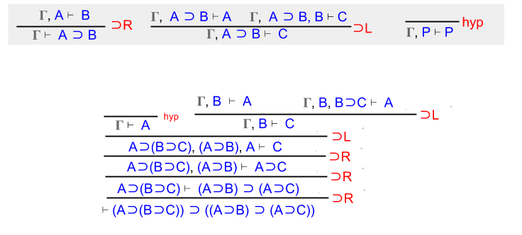
And again, on our newfound B⊃C assumption.
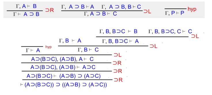
Wait! By now our context by now contains A, B, and C. Each leaf of the proof tree is provable by hyp.
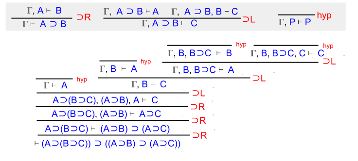
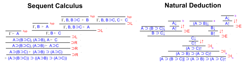
QED. It is instructive to compare this sequent calculus proof with the analogous natural deduction (which we solved together, last time).
Example 2: Distributivity
Show that (A ∨ (B ∧ C)) ⊃ ((A ∨ B) ∧ (A ∨ C)).
The first two steps here are straightforward. Simplify the conjecture string!
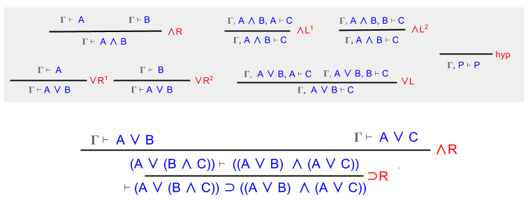
Note that Γ = { A ∨ (B ∧ C) }. Here, we use ∨L to split this assumption into two components:
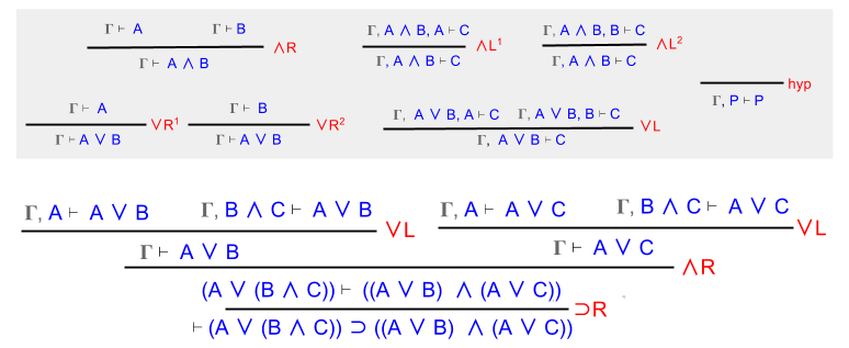
We now have four conjectures to prove. Fortunately, each proof has become trivial:
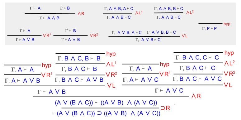
QED.
Takeaways
In this post, we introduced sequent calculus (SC) as an alternative deductive calculus. Sequent calculus makes the notion of context (assumption set) explicit: which tends to make its proofs bulkier but more linear than the natural deduction (ND) style. The two approaches share several symmetries: SC right rules correspond fairly rigidly to ND introduction rules, for example.
If you want to learn sequent calculus for yourself, I recommend solving the converse problems to the two examples above. Specifically,
Until next time!
Part Of: Logic sequence
Content Summary: 500 words, 5 min read
Introduction
Logical systems like IPL have the following ingredients:
We can label propositions in the language of verification.
Introduction and elimination rules can be expressed in this language:

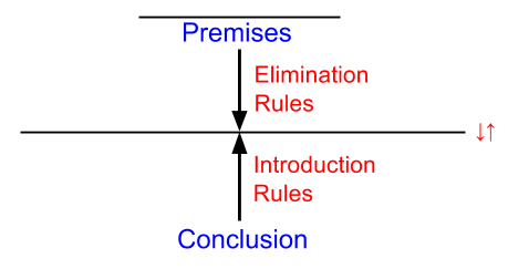
Elimination rules tend to “point down”; introduction rules point up. Roughly, deduction involves applying such rules until the paths meet:
Enough theory! Let’s see how this works in practice.
Exercise One: Implication Exploration
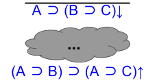
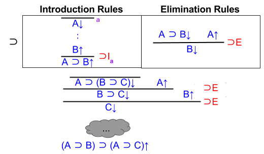
Given A ⊃ (B ⊃ C), show that (A ⊃ B) ⊃ (B ⊃ C).
We can visualize the challenge as follows. The red line indicates common knowledge.
First, let’s apply elimination on the premises:
Next, let’s apply introduction on the conclusion:
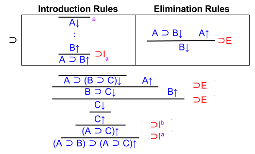
Are we done? No: we have not verified A↑ and B↑. If we had, they would have a red line over them.
To finish the proof, we need to invoke our introduction-rule assumptions.

Proving A↑ is trivial. Proving B↑ requires combining assumptions via elimination.
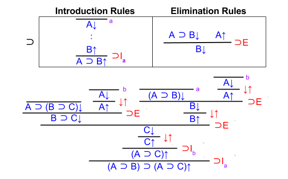
Done. 🙂 Good work!
Exercise for the Reader
Prove the converse is true. Given (A ⊃ B) ⊃ (B ⊃ C), show that A ⊃ (B ⊃ C).
Example 2: Distributivity
In arithmetic, distributivity refers to how addition and multiplication can interleave with one another. It requires that a + (b * c) = (a*b) + (a*c). For example:
Are logical conjunction and disjunction distributive? Let’s find out!
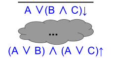
First, let’s introduce conjunction on the conclusion.

Here we reach an impasse. We need to introduce disjunction elimination on the premise. But what should we choose for C?
Let’s set C = A or B.

Filling in the gaps is straightforward. On the right, we eliminate conjunction and retain B. Then we introduce disjunction on both sides.
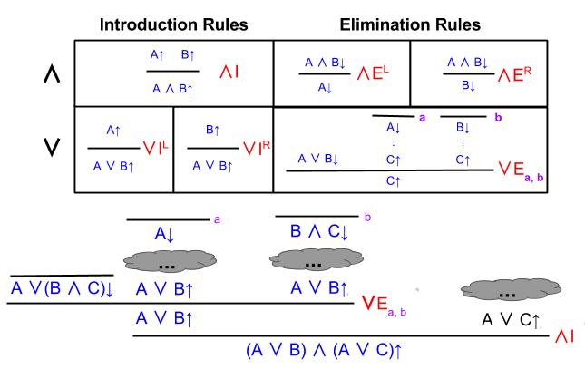
Here is where I originally got stuck. How can we use disjunction elimination?
The way forward becomes easier to grasp, when you remember:
Let’s set the arbitrary elimination symbol “C” equal to A or C:
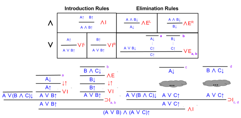
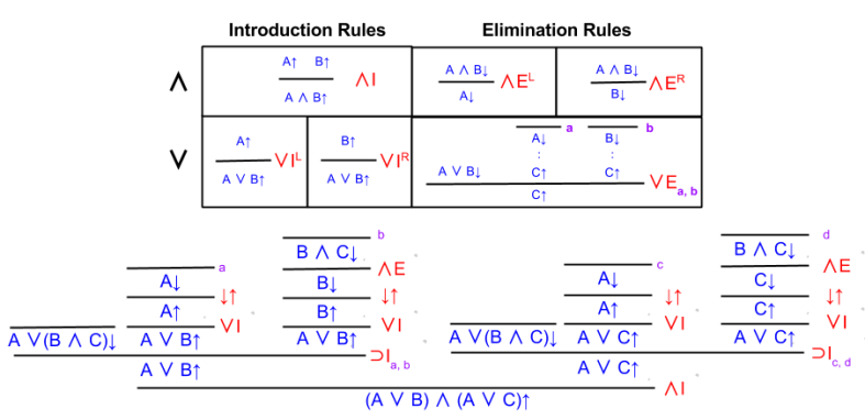
From here, the solution is straightforward.
Exercise for the Reader
Prove the converse is true. Given (A ⊃ B) ⊃ (B ⊃ C), show that A ⊃ (B ⊃ C).
Takeaways
In this post, we saw worked examples of deduction. Specifically:
The best way to learn is practice. For the interested reader, I recommend these exercises:
In the latter exercise, you must also “get creative” on how to use disjunction elimination. Instead of choosing an arbitrary C, you must set A^B to a useful value.
… still stuck? Okay, see solution here. 🙂
Until next time.
Part Of: Machine Learning sequence
Content Summary: 900 words, 9 min read
ML is tribal, not monolithic
Research in artificial intelligence (AI) and machine learning (ML) has been going on for decades. Indeed, the textbook Artificial Intelligence: A Modern Approach reveals a dizzying variety of learning algorithms and inference schemes. How can we make sense of all the technologies on offer?
As argued in Domingos’ book The Master Algorithm, the discipline is not monolithic. Instead, five tribes have progressed relatively independently. What are these tribes?
Expert readers may better recognize these tribes by their signature technologies:
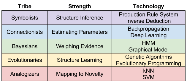
In fact, my blog can be meaningfully organized under this research landscape.
History of Influence
Here are some historical highlights in the development of artificial intelligence.
Symbolist highlights:
Connectionist highlights:
Bayesian highlights:
Evolutionary highlights
Analogizer highlights
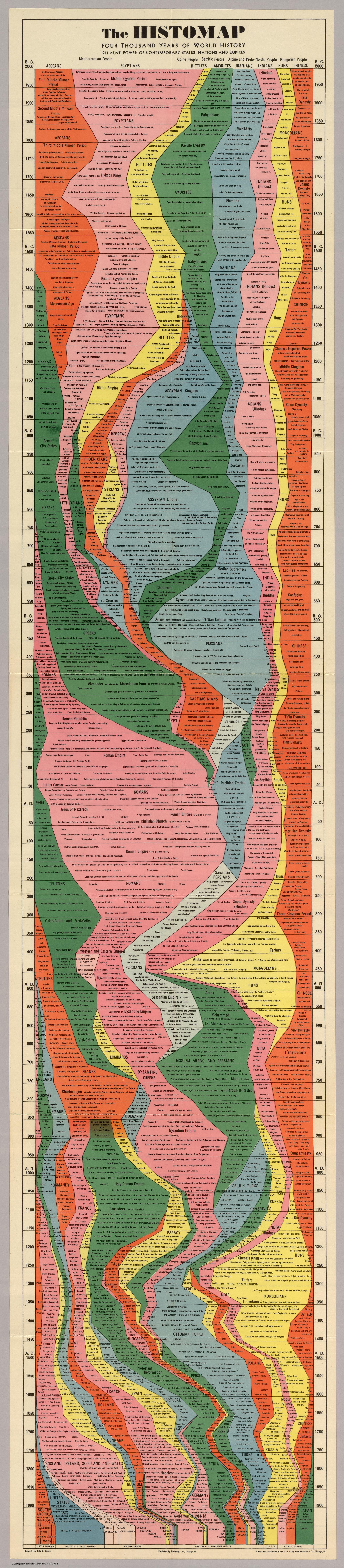
We can summarize this information visually, by creating an AI version of the Histomap:
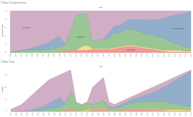
These data are my own impression of AI history. It would be interesting to replace it with real funding & paper volume data.
Efforts Towards Unification
Will there be more or fewer tribes, twenty years from now? And which sociological outcome is best for AI research overall?
Theory pluralism and cognitive diversity are underappreciated assets to the sciences. But scientific progress is often heralded by unification. Unification comes in two flavors:
Perhaps AI progress will mirror revolutions in physics, like when Maxwell unified theories of electricity and magnetism.
Symbolists, Connectionists, and Bayesians suffer from a lack of stability, generality, and creativity, respectively. But one tribe’s weakness is another tribe’s strength. This is a big reason why unification seem worthwhile.
What’s more, our tribes possesses “killer apps” that other tribes would benefit from. For example, only Bayesians are able to do causal inference. Learning causal relations in logical structure, or in neural networks, are important unsolved problems. Similarly, only Connectionists are able to explain modularity (function localization). Symbolist and Bayesian tribes are more normative than Connectionism, which makes their technologies tend towards (overly?) universal mechanisms.
Symbolic vs Subsymbolic
You’ve heard of the symbolic-subsymbolic debate? It’s about reconciling Symbolist and Connectionist interpretations of neuroscience. But some (e.g., [M01]) claim that both theories might be correct, but at different levels of abstraction. Marr [M82] once outlined a hierarchy of explanation, as follows:
One theory, supported by [FP98] is that Symbolist architectures (e.g., ACT-R) may be valid explanations, but somehow “carried out” by Connectionist algorithms & representations.

I have put forward my own theory, that Symbolist representations are properties of the Algorithmic Mind; whereas Connectionism is more relevant in the Autonomic Mind.
This distinction may help us make sense for why [D15] proposes Markov Logic Networks (MLN) as a bridge between Symbolist logic and Bayesian graphical models. He is seeking to generalize these technologies into a single construct; in the hopes that he can later find a reduction of MLN in the Connectionist paradigm. Time will tell.
Takeaways
Today we discussed five tribes within ML research: Symbolists, Connectionists, Bayesians, Evolutionaries, and Analogists. Each tribe has different strengths, technologies, and developmental trajectory. These categories help to parse technical disputes, and locate promising research vectors.
The most significant problem facing ML research today is, how do we unify these tribes?
References
Followup To: Logic Structure: Connectives in IPL
Part Of: Logic sequence
Content Summary: 300 words, 3 min read
Motivations
Last time, we looked at Intuitionistic Propositional Logic (IPL). In IPL, there are five connectives, and hence five introduction-elimination pairs:
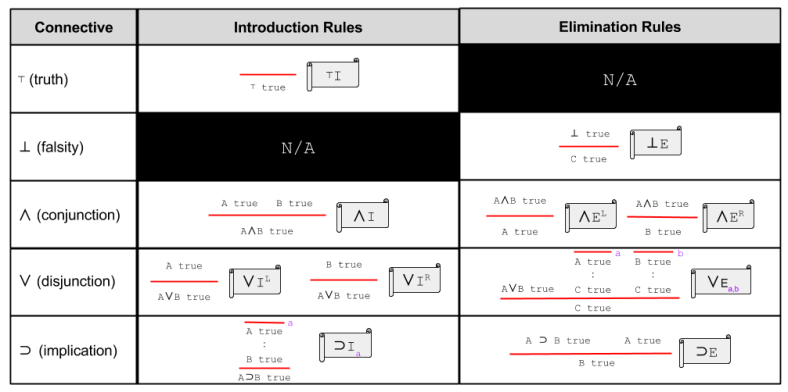
What if you had to design a new logic from scratch? Suppose we were to invent five new connective symbols. Would you start by defining their introduction rule, and use these to infer elimination? Or would you instead define elimination first?
This choice reflects different ways to interpret the semantics of logic:
But if introduction and elimination rules agree, then a logical system has harmony.
How do we evaluate harmony in practice? Harmony is defined as two propositions:
Demonstrating Harmony in IPL
We can show that conjunction rules exhibit harmony.

Note that we have only shown soundness for left-elimination. But demonstrating soundness for right-elimination is highly analogous.
Implication rules also exhibit harmony.

So does disjunction.
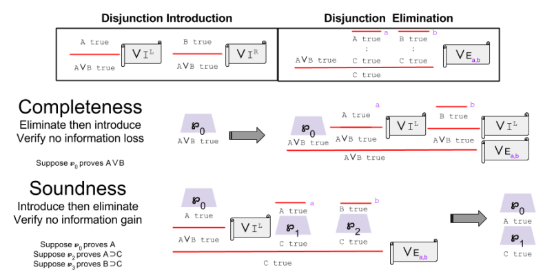
It is trivial to demonstrate the harmony of truth and falsity. Thus, we can say that IPL, as a formal system, has harmony.
Takeaways
In this article, we have discussed harmony, which helps us evaluate how useful a given formal system is. This notion may seem straightforward in IPL; however, it will prove useful in designing new logics, such as linear logic.
Another more subtle point to consider is that the soundness demonstration also seems to reflect a logic of simplification. This point will return when we discuss the Curry-Howard-Lambek correspondence, and the deep symmetries between logic and computation.
Until next time.
Part Of: Logic sequence
Content Summary: 1000 words, 10 min read.
Today, we look at the Zebra Puzzle (aka Einstein Puzzle). According to legend, Albert Einstein invented this as a child, and claimed that 98% of the human population cannot solve it.
Let’s see if we are in the 2%.
The Puzzle
Five men of different nationalities and with different jobs live in consecutive houses on a street. These houses are painted different colors. The men have different pets and have different favorite drinks. The following rules are provided:
Who owns a zebra? And whose favorite drink is mineral water?
To answer this problem, we must learn 5 house-nation-color-drink-pet-job combinations. A solution might look like this:
But this solution is incorrect: it violates Rule 6: “The green house immediately to the right of the white one.”
How do we find a solution that doesn’t violate any of our constraints? Does one even exist? Or is this set of constraints not satisfiable?
Formalizing Logical Structure
Words are distracting. Let’s use symbols instead.
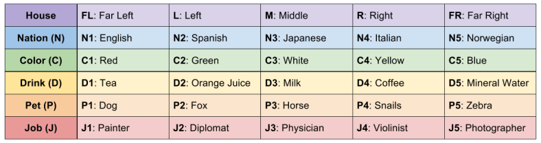
With this code, we can write the above solution as a matrix.

We can also formalize our constraints.

These constraints are ugly. Let’s write them in matrix form instead!

Constraint Satisfaction as a Jigsaw Puzzle
We can use the above constraints to visually check satisfiability. Whereas before you had to parse the meaning of Rule 6 verbally, now you can just inspect whether there is a visual match between rule and solution.

One way to determine satisfiability is to perform these checks until you find a viable solution. But this is computationally expensive: there are 25 billion solutions. Instead of inspecting every possible solutions, why don’t we generate one solution?
How? Since our Rules are used for solution-checking, why can’t we use them for solution-building?
On this view, solution building takes on the flavor of a jigsaw puzzles. Each constraint is a puzzle piece, from these ingredients we construct the solution.
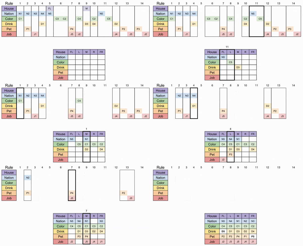
Unfortunately, there is more than one way to solve a 5×5 jigsaw puzzle. Let me show you one way to solve this one. We will be use choice minimization to simplify our lives: try to play the move with the fewest degrees of freedom.
Solution: Path A
Rule 5 and 9 relate to the houses, they are easy to apply.
After these, the Rule 11 puzzle piece fits unambiguously.

Let’s apply Rule 6 next. That jigsaw piece can fit in two locations, the M+R columns, or the R + FR columns. Gotta choose one: let’s select the former. After that move, Rule 10 fits unambiguously.
The FR column is the only place that has an unclaimed nation and color: Rule 1 must go there. similarly, the FL column is the only available spot for Rule 8.
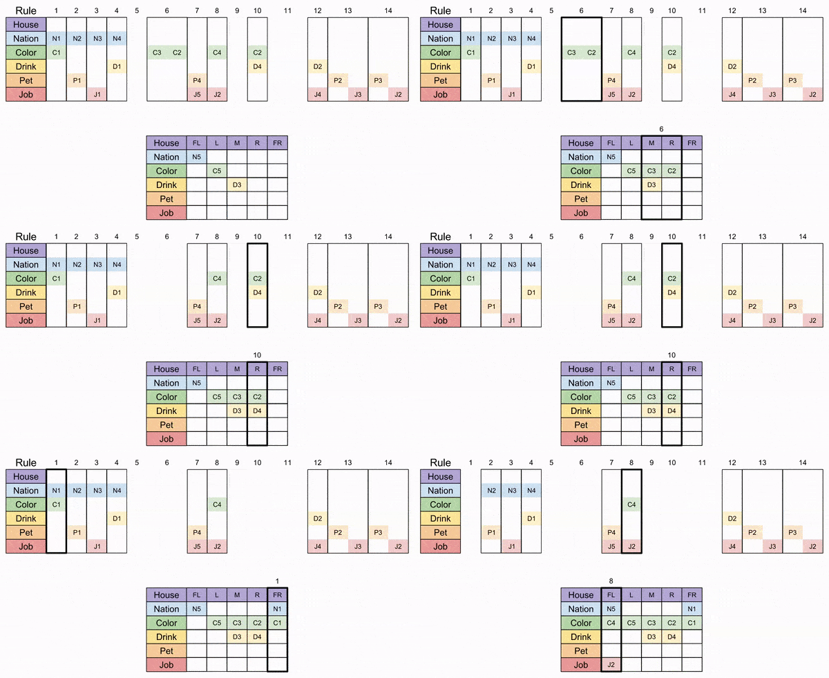
Here we can apply Rule 14 (the original clue’s wording “The horse is in a house next to that of the diplomat” means that the puzzle piece can be flipped horizontally).
After that, only column L can accommodate Rule 4. Then FR must accept Rule 12.

Disaster! Consider Clue 2, 3, and 7. These rules are mutually exclusive (they have at least one row in common with one another), and have overlapping domains (they all cannot fit in FL, but must fit in either M or R).
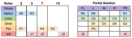
This is the pigeonhole principle: just as three pigeons cannot fit into two holes, there is no way to reach a solution.
Does that mean the puzzle is unsolvable? No, it means we explore other choices.
Solution: Path B
Let’s return to the other possible placement of Rule 6. Instead of putting it in M+R columns, we’ll put it in R+FR. Then, Rules 10, 1, 8, and 14 follow inevitably (each has precisely one choice).

Here we face another choice: do we put puzzle piece 4 in the left or right house? Let’s choose the right house. Then, Rule 12 and Rule 3 follow logically.

Alas! Another disaster. Rule 2 doesn’t fit. 😦
Solution: Path C
Retrace our steps! The last choice we made was Place(4, R). What if we place it in the left house instead?

To our delight, we now see that Path 2b is the only correct logical journey through our puzzle. The concluding steps are given below, and the desired quantities are shown in the “missing” tiles.
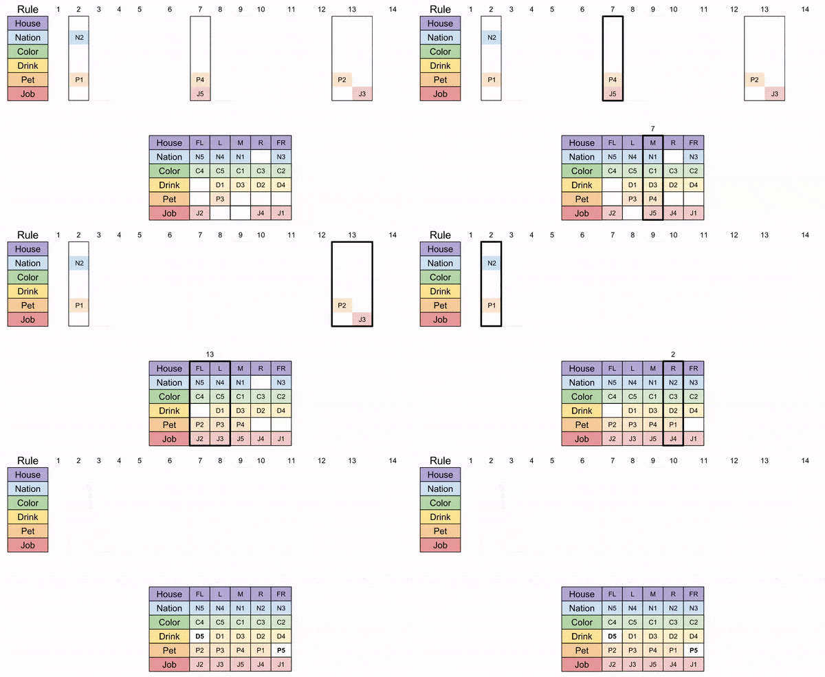
Recall the original questions:
Who owns a zebra (P5)? Whose favorite drink is mineral water (D5)?
Our symbol table can translate our answer:
The Japanese man (N3) owns the zebra, and the Norwegian (N5) drinks mineral water
Implications
The above solution is nothing more to solving a 5×5 jigsaw puzzle. I suspect this technique will only become clear with practice. Go solve Einstein’s Riddle on your own, or one of these variants!
For the solution above, it is helpful to review our search history. Remarkably, we only faced two choices in our solution. When one branch failed, we turned out attention to other branches. This is known as recursion, and will be the subject of another blog post.

Many programming solutions exist for these kinds of problems. In practice, libraries can be used to write more concise solvers.
This kind of problem is called propositional satisfiability (SAT), or constraint programming (CP), although these two disciplines differ in subtle ways.
As we will see next time, SAT problems are at the root of complexity theory and artificial intelligence. Until then.



 Fewer Lacunae