Complementary Learning Systems

Part Of: Demystifying Memory sequence
Content Summary: 1000 words, 10 min read

1.

Your brain is constantly keeping track of the world and your body. It represents these ever-changing environments by patterns of neural activation. Knowledge is not kept in the neurons themselves, but in the connections between neurons.

Sometimes, the brain will discover useful regularities in the environment, and store these patterns for later use. This is long-term memory. We shall concern ourselves with five kinds of long-term memory:

  1. Episodic: ability to remember events or episodes (e.g., dinner last Tuesday night)
  2. Semantic: ability to remember facts and concepts (e.g., hands have five fingers)
  3. Procedural: ability to develop skills (e.g., playing the piano).
  4. Behavioral: ability to remember stimulus-outcome pairs (e.g., bell means food)
  5. Emotional: ability to remember emotional information (e.g., she is always angry).

These memory systems are computed in different areas of the brain.

  1. Episodic memories are computed by the hippocampus
  2. Semantic memories are computed by the association neocortex
  3. Procedural memories are computed by the somatosensory neocortex
  4. Behavioral memories are computed by the basal ganglia
  5. Emotional memories are computed by the central amygdala

Only episodic and semantic memory are directly accessible to consciousness (i.e., working memory). The others are just available to the autonomous mind.

CLS- Categories of Long-Term Memory (1)

2.

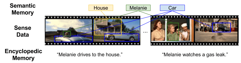
We have previously described conscious experience as a mental movie. But, unlike a normal theater, consciousness has several screens, each of which playing a different sense modality. visual, audio information etc. Call this the multimodal movie.

Semantic memory come in two forms: encyclopedic memory (abstract descriptions of events) and conceptual memory (concepts and their inter-relationships). Both abstractions are derived from the movie, by removing redundant information.
CLS- Episodic vs Semantic Memory

Mind wandering is the tendency of animals to recall past experiences. But why does mind wandering resurrect the details of what was seen, heard, smelled, touched? Why not simply use the plot summary (encyclopedic memory) instead?

Why does episodic memory exist at all?

3.

Henry Molaison was born on February 26, 1926. As a child, he suffered from epilepsy.

CLS- Patient HM (2)

His doctors removed what they thought to be the source of the seizures: the hippocampus. After the surgery, Henry still recognized objects, was able to solve puzzles, even had the same IQ. He had a rich emotional life, and could learn new skills (e.g., to play the piano). But he was completely incapable of forming new episodic memories. Henry (i.e., Patient HM) was locked in a 5 minute loop, never remembering prior events.

Let’s imagine different kinds of amnesia Henry might have experienced.

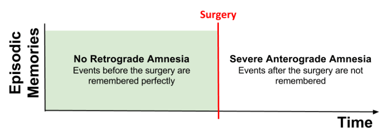
Scenario 1. Henry has no retrograde amnesia (old memories were unperturbed), but suffers severe anterograde amnesia (unable to create new memories). From this data, we might conclude that the hippocampus creates, but does not store, episodic memories.
CLS- HM Amnesia Pattern v1 (1)

Scenario 2. Henry experiences both severe retrograde and anterograde amnesia. From this data, we might conclude that the hippocampus creates and stores episodic memories.

CLS- HM Amnesia Pattern v2 (2)

Neither scenario actually happened. Instead, Henry experienced temporally graded retrograde amnesia:

CLS- HM Amnesia Pattern v3 (2)

This shows that, while the hippocampus creates and stores episodic memories, these memories are eventually copied elsewhere. This process is called consolidation. Hippocampal damage destroy memories that have not yet been consolidated. 

But why should the brain copy memories? This seems inefficient. And why does this process take years, even decades?

4.

The connectionist paradigm models the brain as a neural networkThe AB-AC task illustrates a challenge for connectionism. It goes as follows:

You want to associate stimulus A with response B. For example, when you hear “chair”, you should say “map”. There are many such associations (Chair-Map, Book-Dog, Car-Idea). This is the AB list.

After you achieve 100% recall on the AB list , a new set of stimulus-response words are given: the AC list. You want to learn both. However, the AB and AC lists have the same stimuli paired with novel responses (e.g. Chair-Printer, Book-Flower, Car-Shirt).

How well do humans and connectionist models do against this task? Let’s find out! The following graphs take place after the AB list has been learned perfectly. Y-axis is %correct, x-axis is number of exposures to the AC list.

CLS- Catastrophic Interference (2)

Consider the left graph. Dotted line is AC recall over time. Humans were able to learn the AC list. The solid line shows AB list performance. As humans learned AC associations, their AB performance suffered a little, from 100 to 60%. This is moderate interference.

Consider the right graph. Dotted line shows that the model is able to learn the AC list, just like the human. But solid line shows that AB recall very quickly drops to 0%. This is catastrophic interference.

Catastrophic interference occurs when the AB list and AC list are learned separately (focused learning). But what if you learn them at the same time? More specifically, what if you train against a shuffled set of AB and AC associations (interleaved learning)?
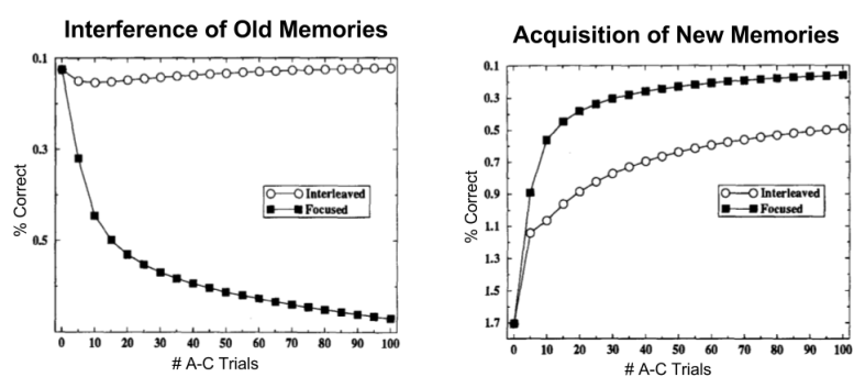
CLS- Interleaved vs Focused Learning (2)

On the left, focused learning (black squares) shows catastrophic interference against AB memories, as before. But interleaved learning (white dots) show zero interference!

On the right, we see another consequence of interleaved learning: new memories are acquired much more slowly.

5.

We are ready to put the puzzle together.

Catastrophic interference is an inevitable consequence of systems that employ highly-overlapping distributed representations, despite the fact that such systems have a number of highly desirable properties (e.g., the ability to perform generalization and inference).

This problem can be addressed by employing a structurally distinct system with complementary learning properties: sparse, non-overlapping representations that are highly robust to interference from subsequent learning. Such a sparse system by itself would be like an autistic savant: good at memorization but unable to perform everyday inferences. But when paired with the highly overlapping system, a much more versatile overall system can be achieved.

The neocortex and hippocampus comprise these learning systems:

CLS- Two Component Model

First introduced in 1995, Complementary Learning System (CLS) theory predicts a wide range of extant biological, neuropsychological, and behavioral data. It explains why the hippocampus exists, why it performs consolidation, and why consolidation takes years to complete.

The CLS theory was first presented in [M95]. Data in section 4 taken from that paper. Section 5 quotes liberally from [O11].

  • [M95] McClelland et al (1995). Why There Are Complementary Learning Systems in the Hippocampus and Neocortex: Insights From the Successes and Failures of Connectionist Models of Learning and Memory
  • [O11] O’Reilly et al (2011). Complementary Learning Systems
The Tripartite Mind

Part Of: Neural Architecture sequence
Content Summary: 700 words, 7 min read

Dual-Process Theory

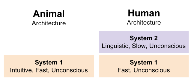
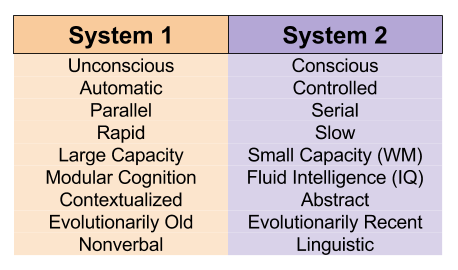
Dual process theory identifies two modes of human cognition: a fast, parallel System 2 and a slow, serial System 1.

Linguistic Implications- Dual Process Theory

This distinction can be expressed phylogenetically:

Tripartite Mind- Dual-Process Theory Phylogeny (2)

But this is incorrect. We know that engine of consciousness is the extended reticular-thalamic activating system (ERTAS), which implements feature integration by phase binding.  Mammalian brains contain this device. Also, behavioral evidence indicate that non-human animals possess working memory and fluid intelligence[C13].

Conscious, non-linguistic animals exist. We need a phylogeny that accepts this fact.

The Tripartite Mind

Let’s rename System 1, and divide System 2 into two components.

  • The Autonomous mind is a subsymbolic neural network.
  • The Algorithmic Mind constructs perceptual object via the Global Workspace.
  • The Linguistic Mind applies linguistic processing to conscious contents.

This allows us to conceive of conscious, non-verbal mammals:

Linguistic Musings- Architectural Phylogeny (1)

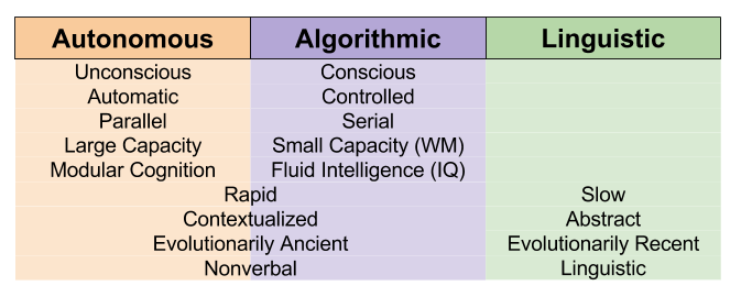
This lets us refresh our view of property dissociations:

Tripartite Mind- TPM Property Dissociations (1)

Most dual-process theorizing (for example, our theory of moral cognition) maps neatly to the autonomous and linguistic mind, respectively.

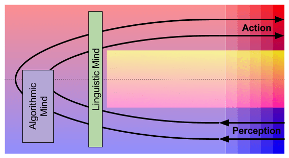
But the Tripartite Mind theory cannot bear the weight of all behavioral phenomena. For that, we need the more robust language of two loops. In fact, we can marry these two theories as follows:

Tripartite Mind- Cybernetics Interpretation

This diagram reflects the following facts:

  • The Autonomous Mind constitutes most of the brain.
  • The Algorithmic Mind is perceptual, and processes Autonomic representations.
  • The Linguistic Mind receives Algorithmic (but not Autonomic) information.

Boundaries on the Linguistic Mind

The Linguistic Mind creates cultural knowledge. It is the technology underlying the invention of agriculture, calculus, and computational neuroscience. It is hard to see how such a device could be not only biased, but in some respects completely blind.

But the Linguistic Mind does not have access to raw sensorimotor signals. It only has access to the intricately curated working memory. You cannot communicate mental experiences outside of working memory. You can try, but that would be confabulation (unintentional dishonesty). As [NW77] describe in their seminal paper Telling more than we can know, in practice, human beings are strangers to themselves.

The evidence suggests that working memory does not contain any information about your judgments and decision making. All attempts to describe this aspect of our inner life fail. Introspection on these matters cannot secure direct access to the truth of the matter. Rather, we guess at our own motives, using the exact same machinery we use to interpret the behavior of other people. For more on the Interpretive Sensory Access theory of introspection [C10], I recommend this lecture.

Sociality and the Linguistic Mind

Per the Social Brain Hypothesis [D09], humans are not more intelligent than other primates; we are rather more social. In other words, the Linguistic Mind is a social invention, which facilitates the construction of cultural institutions which allow propriety frames to be synchronized more explicitly.

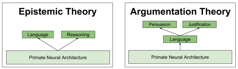
On the argumentative theory of reasoning, social reasoning is not independent of language. It is the purpose of language.

Argumentative Reason- Module Evolution (2)

While the Linguistic Mind evolved to satisfy social selection pressures, not all primate sociality is linked to this device. Social mechanisms have arrived in stages:

  • Primary emotions as social behavior network can be traced back to ray-finned fish.
  • In New World primates, body language evolved as an extension to our autonomic nervous system, as described in the polyvagal theory. [P03]
  • Certain human-specific social mechanisms evolved within the neuroimmune axis as a defense mechanism to parasites [TF14].

All of these mechanisms can be attributed to the Autonomous Mind. But since the Linguistic Mind is driven by our motivation apparatus (just like everything else in the brain), its behavior is sensitive to the wishes of these “lower” modules. This doesn’t contradict our earlier assumption that its content is divorced from Autonomous data.

References

  • [C13] Carruthers 2013. Evolution of working memory.
  • [C10] Carruthers 2010. Introspection: Divided and Partly Eliminated
  • [TF14] Thornhill, Fincher (2014). The Parasite-Stress Theory of Sociality, the Behavioral Immune System, and Human Social and Cognitive Uniqueness.
  • [P03] Porges (2003). The Polyvagal Theory: phylogenetic contributions to social behavior
  • [D09] Dunbar (2009). The social brain hypothesis and its implications for social evolution

OLS Estimation via Projection

Part Of: Machine Learning sequence
Content Summary: 800 words, 8 min read

Projection as Geometric Approximation

If we have a vector b and a line determined by vector a, how do we find the point on the line that is closest to b?

OLS- Geometry of Projection

The closest point p is at the intersection formed by a line through b that is orthogonal to a. If we think of p as an approximation to b, then the length of e = b - p is the error of that approximation.

a^T e = a^T (b - ax) = 0

This formula captures projection onto a vector. But what if you want to project to a higher dimensional surface?

Imagine a plane, whose basis vectors are a_1 and a_2. This plane can be described with a matrix, by mapping the basis vectors onto its column space:

A = \begin{bmatrix} a_1 & a_2 \end{bmatrix}

Suppose we want to project vector b onto this plane. We can use the same orthogonality principle as before:

A^Te = A^T(b-Ax) = 0

A^TAx = A^Tb

Matrices like A^TA are self-transpositions. We have shown that such matrices are square symmetric, and thereby contain positive, real eigenvalues.

We shall assume that the columns of A^TA are independent, and it thereby is invertible. The inverse thereby allows us to solve for x:

(A^TA)^{-1}(A^TA)x = (A^TA)^{-1}A^Tb

x = (A^TA)^{-1}A^Tb

Recall that,

p = Ax = A(A^TA)^{-1}A^Tb

Since matrices are linear transformations (functions that operate on vectors), it is natural to express the problem in terms of a projection matrix P, that accepts a vector b, and outputs the approximating vector p:

p = Pb

By combining these two formula, we solve for P:

P = A(A^TA)^{-1}A^T

Thus, we have two perspectives on the same underlying formula:

OLS- Regression Functions via Matrices (1)

Linear Regression via Projection

We have previously noted that machine learning attempts to approximate the shape of the data. Prediction functions include classification (discrete output) and regression (continuous output).

Consider an example with three data points. Can we predict the price of the next item, given its size?

OLS- Regression Function Setup

For these data, a linear regression function will take the following form:

\psi : Size \rightarrow Price

\psi(Size) = \beta_0 + \beta_1 Size

We can thus interpret linear regression as an attempt to solve Ax=b:

OLS- Linear Algebra Regression Matrix

In this example, we have more data than parameters (3 vs 2). In real-world problems, it is an extremely common predicament. It yields matrices with may more equations than unknowns. This means that Ax=b has no solution (unless all data happen to fall on a straight line).

If exact solutions are impossible, we can still hope for an approximating solution. Perhaps we can find a vector p that best approximates b. More formally, we desire some p = A\bar{x} such that the error e = b-p is minimized.

Since projection is a form of approximation, we can use a projection matrix to construct our linear prediction function \psi : Size \rightarrow Price.

OLS- Least Squares Fundamental Spaces

A Worked Example

The solution is to make the error b-Ax as small as possible. Since Ax can never leave the column space, choose the closest point to b in that subspace. This point is the projection p. Then the error vector e = b-p has minimal length.

To repeat, the best combination p = Ax is the projection of b onto the column space. The error is perpendicular to that subspace. Therefore e = b-p is in the left nullspace:

Ax = b

A^TA = \begin{bmatrix} 1 & 1 & 1 \\ 1 & 2 & 3 \\ \end{bmatrix} \begin{bmatrix} 1 & 1 \\ 1 & 2 \\ 1 & 3 \\ \end{bmatrix} = \begin{bmatrix} 3 & 6 \\ 6 & 14 \\ \end{bmatrix}

We can use Guass-Jordan Elimination to compute the inversion:

(A^TA)^{-1} = \begin{bmatrix} 7/3 & -1 \\ -1 & 1/2 \\ \end{bmatrix}

A useful intermediate quantity is as follows:

(A^TA)^{-1}A^T = \begin{bmatrix} 7/3 & -1 \\ -1 & 1/2 \\ \end{bmatrix} \begin{bmatrix} 1 & 1 & 1 \\ 1 & 2 & 3 \\ \end{bmatrix} = \begin{bmatrix} 4/3 & 1/3 & -2/3 \\ -1/2 & 0 & 1/2 \\ \end{bmatrix}

We are now able to compute the parameters of our model, \bar{x}:

\bar{x} = \left[ (A^TA)^{-1}A^T \right] b = \begin{bmatrix} 4/3 & 1/3 & -2/3 \\ -1/2 & 0 & 1/2 \\ \end{bmatrix} \begin{bmatrix} 1 \\ 2 \\ 2 \\ \end{bmatrix} = \begin{bmatrix} 2/3 \\ 1/2 \\ \end{bmatrix}

These parameters generate a predictive function with the following structure:

\psi : Size \rightarrow Price

\psi(Size) = \frac{2}{3} + \frac{1}{2}Size

These values correspond with the line that best fits our original data!

Wrapping Up

Takeaways:

  • In linear algebra, projection approximates a high-dimensional surface in a lower-dimensional space. The projection error can be measured.
  • In linear regression, we usually cannot solve Ax=b, because there tends to be more data than parameters (b is not in the column space)
  • We can find the closest vector in the column space by projecting onto b, and minimizing the projection error.
  • Thus, the operation of projection can be used to perform parameter estimation, and produce a model that best approximates the training data.

Related Resources:

The Argumentative Theory of Reason

Part Of: Demystifying Language sequence
Content Summary: 1200 words, 12 min read.

The Structure of Reason

Learning is the construction of beliefs from experience. Conversely, inference predicts experience given those beliefs.

Reasoning refers to the linguistic production and evaluation of an argument. Learning and inference are ubiquitous across all animal species. But only one species are capable of reasoning: human beings.

Argument can be understood by the lens of deductive logic. Logical syllogisms are a calculus that maps premises to conclusions. An argument is valid if the conclusions follow from the premises. An argument is sound if it is valid, and its premises are true.

Premises can be evaluated directly via intuition. The relationship between argument structure and intuition parallels decision trees versus evaluative functions.

Two Theories of Reason

Why did reasoning evolve? What is its biological purpose? Consider the following theories:

  1. Epistemic theoryreasoning is an extension of our individual cognitive powers. 
  2. Argumentative theory: reasoning is a device for social communication.

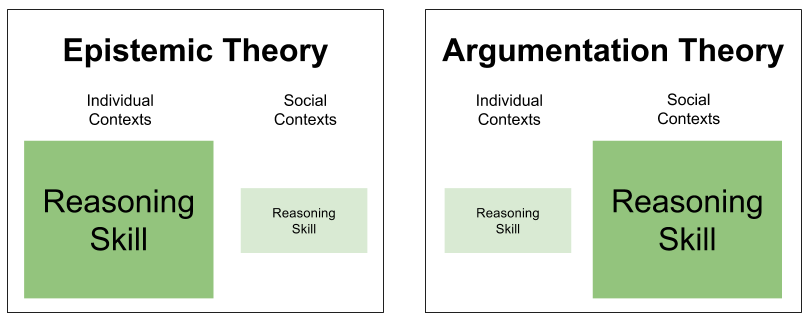
One way to adjudicate these rival theories is to examine domain gradients. Roughly, a biological mechanism performs optimally when situated in contexts for which they were originally designed. Our cravings for sugars and fats mislead us today, but encourage optimal foraging in the Pleistocene epoch.

Reasoning is used in both individual and social contexts. But our theories disagree on which is the original domain. Thus, they generate opponent predictions as to which context will elicit the most robust performance.

Argumentative Reason- Domain Gradients (1)

Here we see our first direct confirmation of the argumentative theory: in practice, people are terrible at reasoning in individual contexts. Their reasoning skills become vibrant only when placed in social contexts. It’s a bit like Kevin Malone doing mental math. 🙂

Structure of Argumentative Reason

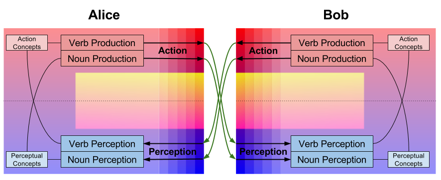
All languages ever discovered contain both nouns and verbs. This universal distinction reflects the brain’s perception-action dichotomy. Nouns express perceptual concepts, and verbs express action concepts.

Recall that natural language has two processes: speech production & speech comprehension. These functions both accept nouns and verbs as arguments. Thus, we can express the cybernetics of language as follows:
Argumentative Reason- Cybernetics of Language

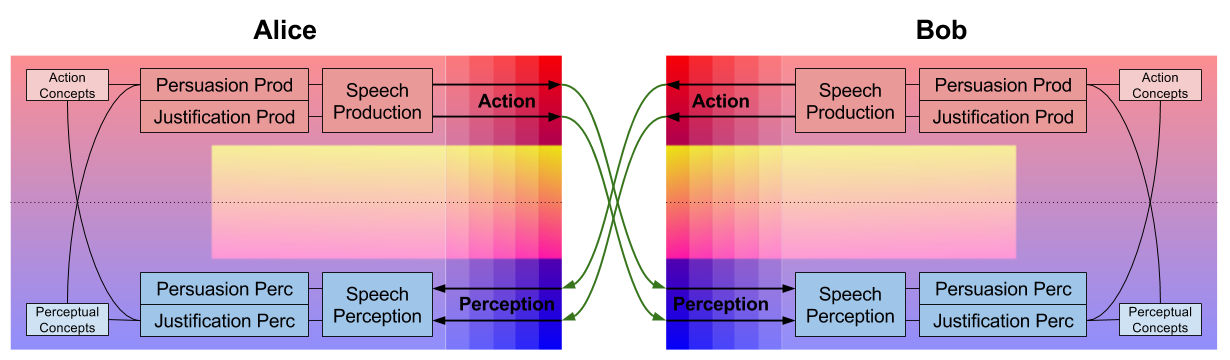
Argumentative reasoning is a social extension of the faculty of language. It consists of two processes:

  1. Persuasion deals with arguments to support beliefs. 
  2. Justification deals with reasons to justify our actions.

Persuasion and justification draw on perceptual and action concepts, respectively. Thus, the persuasion-justification distinction mirrors the noun-verb distinction, but at a higher level of abstraction. Here is our cybernetics of reasoning diagram.

Argumentative Reason- Cybernetics of Reason

We return to phylogeny. Why did reasoning-as-argumentation evolve?

For communication to persist, it must benefit both senders and receivers. But stability is often threatened by senders who seek to manipulate receivers. We know that humans are gullible by default. Nevertheless, our species does possess lie detection devices. 

The evolution of argumentative reason was shaped by a similar set of ecological pressures as that of language. Let me cover these hypotheses in another post.

For now, it helps to think of belief as clothes, serving both pragmatic and social functions. A wide swathe of biases stems from persuasive arguments performing social rather than epistemic ends.  This is not to say that truth is irrelevant to reasoning. It is simply not always the dominant factor.

On Persuasion

Persuasion processes involve arguments about beliefs. It has two subprocesses: argument production (listener persuasion) and argument evaluation (argument quality inspection). These two processes are locked in an evolutionary arms race, developing ever more sophisticated mechanisms to defeat the other.

Argument production is responsible for the two most damning biases in the human repertoire. There is extensive evidence that we are subject to confirmation bias: the attentional habit to preferentially examine evidence that helps our case. We are also victim to motivated reasoning, which biases our judgments towards our self-interest. We often describe instances of motivated reasoning as hypocrisy.

Consider the following example:

There are two tasks one short & pleasant, the other long & unpleasant. Selectors are asked to select their task, knowing that the other task is giving to another participant (the Receiver). Once they are done with the task, each participant states how fair the Selector has been. It is then possible to compare the fairness ratings of Selectors versus those of the Receivers.

Selectors rate their decisions as more fair than the Receivers, on the average. However, if participants are distracted when they asked their fairness judgments, the ratings were identical and showed no hint of hypocrisy. If reasoning were not the cause of motivated reasoning but the cure for it, the opposite would be expected.

In contrast to production, argument evaluation involves two subprocesses: trust calibration and coherence checking. The ability to distrust malevolent informants has been shown to develop in stages between the ages of 3 and 6.

Coherence checking is less self-serving than production mechanism. In fact, it is responsible for the phenomenon of truth wins. For example, in group puzzles the person whoever stumbles on the solution will successfully persuade her peers, regardless of her social standing. In practice, good arguments tend to be more persuasive than bad arguments. 

On Justification

Justification processes involve reasons about behavior. This is not to be confused with motivations for behavior, which happen at the subconscious level. In fact, there is evidence to suggest that the reasons we acquire by introspection are not true. It has been consistently observed that attitudes based on reasons are much less predictive of future behaviors (and often not predictive at all) than were attitudes stated without recourse to reasons.

The justification module produces reason-based choice; that is, we tend to choose behaviors that are easy to justify to our peers. Reason-based choice explains an impressive number of documented human biases. For example,

The sunk cost fallacy is the tendency to continue an endeavor once an investment has been made. It doesn’t occur in children or non-human animals. If reasoning were not the cause of this phenomenon but the cure for it, the opposite would be expected.

The disjunction effect, endowment effect, and decoy effect can similarly be explained in terms of reason-based choice.

This is not to say that justification is insensitive to the truth. Better decisions are usually easier to justify. But when a more easily justifiable decision is not a good one, reasoning still drives us towards ease of justification.

Theory Evaluation

I was initially skeptical of the argumentative theory because it felt “fashionable” in precisely the wrong sense, underwritten by postmodern connotations of narrative-is-everything and epistemic nihilism. Another warning flag is that the theory draws from the field of social psychology, which has been quite vulnerable to the replication crisis.

However, the evidential weight in favor of the argumentative theory has recently persuaded me. For a comphrehensive view of that evidence, see [MS11]. I no longer believe argumentative reason entails epistemic nihilism, and I predict its evidential basis will not erode substantially in coming decades.

I am also attracted to the theory because it helps tie together several other theories into a comprehensive meta-theory: The Tripartite Mind. Let me sketch just one of example of this appeal.

The heuristics and biases literature has uncovered a bewildering variety of errors, shortcuts, and idiosyncrasies in human cognition.  Responses to this literature vary widely. But too many voices take such biases as “conceptual atoms”, or fundamental facts of the human brain. Neuroscience can and must identify the mechanisms underlying these phenomena.

The argumentative theory is attractive in that it explains a wide swathe of the zoo.

Argumentative Reason- Bias Explanation (1)

Takeaway

Reason is not a profoundly flawed general mechanism. Instead, it is an efficient linguistic device adapted to a certain type of social interaction.

References

[MS11]. Mercer & Sperber (2011). Why do humans reason? Arguments for an argumentative theory.

Regression vs Classification

Part Of: Machine Learning sequence
Content Summary: 500 words, 5 min read

Motivations

Data scientists are in the business of answering questions with data. To do this, data is fed into prediction functions, which learn from the data, and use this knowledge to produce inferences.

Today we take an intuitive, non-mathematical look at two genres of prediction machine: regression and classification. Whereas these approaches may seem unrelated, we shall discover a deep symmetry lurking below the surface.

Introducing Regression

Consider a supermarket that has made five purchases of sugar from its supplier in the past. We therefore have access to five data points:

Regression Classification- Regression Data (3)

One of our competitors intends to buy 40kg of sugar. Can we predict the price they will pay?

This question can be interpreted visually as follows:

Regression Classification- Regression Prediction Visualization

But there is another, more systematic way to interpret this request. We can differentiate training data (the five observations where we know the answer) versus test data (where we are given a subset of the relevant information, and asked to generate the rest):

Regression Classification- Regression Prediction Schema

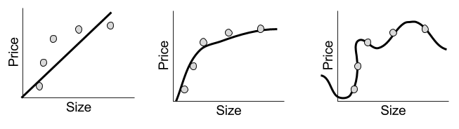
A regression prediction machine will for any hypothetical x-value, predicts the corresponding y-value. Sound familiar? This is just a function. There are in fact many possible regression functions, of varying complexity:

Regression Classification- Simple vs Complex Regression Outputs

Despite their simple appearance, each line represents a complete prediction machine. Each one can, for any order size, generate a corresponding prediction of the price of sugar.

Introducing Classification

To illustrate classification, consider another example.

Suppose we are an animal shelter, responsible for rescuing stray dogs and cats. We have saved two hundred animals; for each, we record their height, weight, and species:
Regression Classification- Classification Data (1)

Suppose we are left a note that reads as follows:

I will be dropping off a stray tomorrow that is 19 lbs and about a foot tall.

A classification question might be: is this animal more likely to be a dog or a cat?

Visually, we can interpret the challenge as follows:

Regression Classification- Classification Prediction Interpretation (2)

As before, we can understand this prediction problem as taking information gained from training data, to generate “missing” factors” from test data:

Regression Classification- Classification Prediction Schema

To actually build a classification machine, we must specify a region-color map, such as the following:

Regression Classification- Simple Classification Output

Indeed, the above solution is complete: we can produce a color (species) label for any new observation, based on whether it lies above or below our line. 

But other solutions exist. Consider, for example, a rather different kind of map:Regression Classification- Complex Classification Boundary

We could use either map to generate predictions. Which one is better? We will explore such questions next time.

Comparing Prediction Methods

Let’s compare our classification and regression models. In what sense are they the same?

Regresssion Classification- Comparing Models

If you’re like me, it is hard to identify similarities. But insight is obtained when you compare the underlying schemas:

Regresssion Classification- Comparing Schema

Here we see that our regression example was 2D, but our classification example was 3D. It would be easier to compare these models if we removed a dimension from the classification example.

Regresssion Classification- 1D Classification (1)

With this simplification, we can directly compare regression and classification:

Regresssion Classification- More Direct Comparison

Thus, the only real difference between regression and classification is whether the prediction (the dependent variable) is continuous or discrete.

Until next time.

The Structure of Ethical Theories

Part Of: Demystifying Ethics sequence
Followup ToAn Introduction To Ethical Theories
See Also: Shelly Kagan (1994). The Structure of Normative Ethics
Content Summary: 700 words, 7 min read

Are Ethical Theories Incompatible?

Last time, we introduced five major ethical theories:

Ethical Theories- Summary

At first glance, we might consider these theories as rivals competing for the status of a ground for morality. However, when discussing these theories, one has a distinct sense that they are simple addressing different concerns.

Perhaps these theories are compatible with one another. But it is hard to see how, because we lack a map of the major conceptual regions of normative ethics, and how they relate to one another.

Let’s try to construct such a map.

Identifying Morally Relevant Factors

There are two major activities in the philosophical discourse about normative ethics: factorial analysis, and foundational theories.

Factorial analysis involves getting clear on which variables affect in our moral judgments. This is the goal of moral thought experiments. By constructing maps from situations to moral judgment, we seek to understand situational factors that contribute to (and compete for control over) our final moral appraisals.

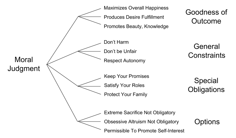
We can discern four categories of factors which bear on moral judgments: Goodness of Outcome, General Constraints, Special Obligations, and Options. We might call these categories factorial genres. Here are some example factors from each genre.

Ethics Taxonomy- Morally Relevant Factors (1)

While conducting factorial analysis, we typically ask questions about:

  1. Relative Strength. Does Don’t Harm always outweigh factors related to outcome?
  2. Explanatory Parsimony. Is Keep Your Promises redundant with Don’t Be Unfair?
  3. Subfactor Elaboration. What does Maximize Overall Happiness mean, exactly?

Constructing Foundational Theories

A foundational mechanism is a conceptual apparatus designed to generate the right set of morally relevant factors. An example of such a theory is contractarianism, which roughly states that:

Morally relevant factors are those which would be agreed to by a social community, if they were placed in an Original Position (imagine you are designing a social community from scratch), and subject to the Veil of Ignorance (you don’t know the details of what your particular role will be).

Thus, our two philosophic activities relate as follows:

Ethical Structure- Factors vs Foundations (2)

These two activities are fueled by different sets of intuitions.

  • Factorial intuitions are identified by appeal to concrete ethical dilemmas.
  • Foundational intuitions are often related to one’s metaethical dispositions.

Let us examine other accounts of foundational mechanisms. These claim that we should accept only morally relevant factors that…

  • …if everyone followed such rules, total well-being would be maximized (rule utilitarianism).
  •  … if the factor was universalized, became like a law of nature, no contradictions would emerge (Kantian universalization).
  • … can be attributed to a being acting purely in self-interest (egoism).

Localizing Ethical Theories in our Map

We can now use this scheme to better understand the space of ethical theories.

Proposition 1. Ethical theories can be decomposed into their foundational and factorial components.

Three of our five ethical theories have the following decomposition:

Ethical Structure- Deconstructing Ethical Theories (1)

Proposition 2. Factorial pluralism is compatible with foundational monism.

Certain flavors of consequentialists, deontologists, consequentialists insist on factorial monism, that only one kind of moral factor really matters.

But as a descriptive matter, it seems that human morality is sensitive to many different kinds of factors. Outcome valence, action constraint, role-based obligations all seem to play in real moral decisions.

Factorial monism has the unpleasant implication of demonstrating some of these factors as misguided. But philosophers are perfectly free to affirm factorial pluralism: that each intuition “genre” are prescriptively justified.

Some examples of one foundational device generating a plurality of genres:

  1. Rule Utilitarianism (rules that maximize societal well-being) could easily generate rules to keep one’s promises.
  2. Kantian Universalization might generate outcome-sensitive moral factors that are immune to contradiction.
  3. People in the Original Position might enter into a contract of general constraints (e.g., human rights).

Takeaways

Are ethical theories truly competitors? One might suspect that the answer is no. Ethical theories seem to address different concerns.

We can give flesh to this intuition by analyzing the structure of ethical theories. They can be decomposed into two parts: factorial analysis, and foundational mechanisms.

  • Factorial analysis provide the list of factors relevant to moral judgments.
  • Foundational mechanisms are hypothesized to generate these moral factors.

Ethical Structure- Factors vs Foundations (2)

Most defenses of foundational mechanisms have them generating a single factorial genre. However, it is possible to endorse factorial pluralism. There is nothing incoherent in the view that e.g., both event outcome and general constraints bear on morality.

This taxonomy allows us to contrast ethical theories in a new way. Utilitarianism can be seen as a theory about the normative factors, contractarianism is a foundational mechanism. Far from being rival views, one could in fact endorse both!