An Introduction To Markov Chains

October 17, 2016May 9, 2017kevinbinz 1 Comment

Part of: Reinforcement Learning sequence
Related to: An Introduction to Linear Algebra
Content Summary: 700 words, 7 min read

Motivation

We begin with an example.

Suppose a credit union classifies automobile loans into four categories: Paid in Full (F), Good Standing (G), Behind Schedule (B), Collections (C).

Past records indicate that each month, accounts in good standing change as follows: 10% pay the loan in full, 10% fall behind on payments, 80% remain in good standing.

Similarly, bad loans historically change every month as follows: 10% are paid in full, 40% return to good standing, 40% remain behind schedule, 10% are sent to collection.

A Markov Chain allows us to express such situations graphically:

Loan statuses are nodes, transition probabilities are arrows.

Markov Property

Formally, a Markov Chain is a tuple (S, P)

A set of states s ∈ S
A transition model P(s’ | s).

At the core of Markov Chains is the Markov Property, which states (for time t = n):

$P(s_n | s_{n-1}, s_{n-2}, \dots, s_0) = P(s_n | P(s_{n-1})$

This is a statement of conditional independence. If I tell you the history of all prior states, and ask you to predict the next time step, you can forget everything except the present state. Informally, a complete description of the present screens off any influence of the past. Thus, the Markov Property ensures a kind of “forgetful” system.

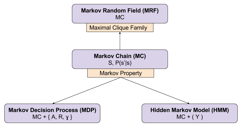
Any model which relies on the Markov Property is a Markov Model. Markov models represent an important pillar in the field of artificial intelligence. Three extensions of Markov Chains are particularly important:

Reinforcement Learning- Markov Models

State Expectations by Unweaving

Let’s imagine a Markov Chain with three states: A, B, and C. If you begin at A, where should you expect to reside in the future?

An intuitive way to approach this question is to”unweave” the Markov Chain, as follows:

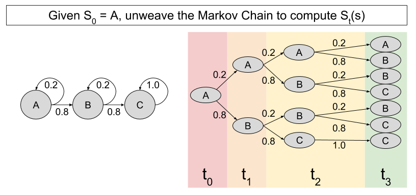
Each branch in this tree represents a possible world. For example, at t₁ there is a 20% chance the state will be A, and an 80% chance the state will be B. Computing expected locations for subsequent timesteps becomes straightforward enough. At t₂, we see that:

There is an (0.2)(0.2) = 4% chance of residing in A.
There is an (0.8)(0.2) + (0.2)(0.8) = 32% chance of residing in B.
There is an (0.8)(0.8) = 64% chance of residing in C.

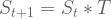
The above computations can be expressed with a simple formula:

$S_t(s) = \sum_{paths}\prod_{edges} P(s|s')$

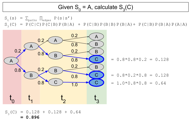
However, these computations become tedious rather quickly. Consider, for example S₃(C):

State Expectations By Linear Algebra

Is there a way to simplify the maths of expectation?

Yes, by approaching Markov Chains through the lens of linear algebra. Conditional probabilities are encoded as transition matrices, as follows:

This representation enables computation of expected location by matrix multiplication:

$S_{t+1} = S_t * T$

We compute expectation timesteps sequentially. By defining a base case and an inductive step, this process qualifies as mathematical induction.

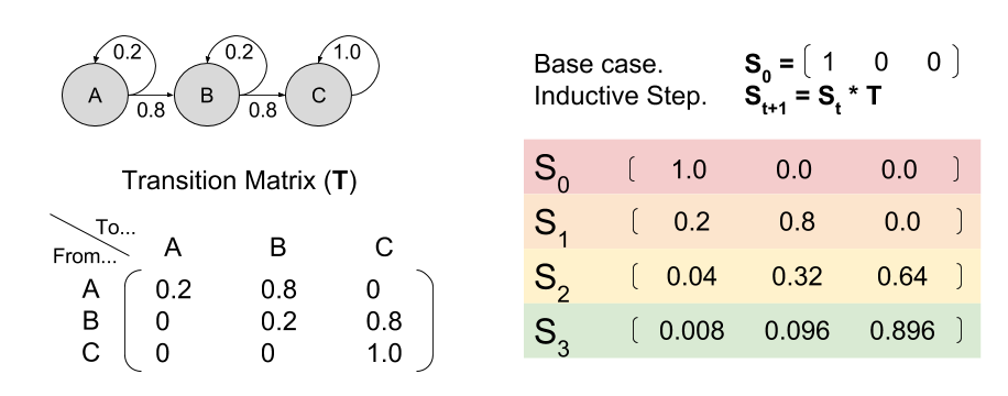
As you can see, these maths are equivalent: S₃(C) = 0.896 in both cases.

Steady-State Analysis

In the above example, C is called an absorbing state. As time goes to infinity, the agent becomes increasingly likely to reside in state C. That is, S_n = [0 0 1] as n→∞. This finding generalizes. Every Markov Chain that contains a (reachable) absorbing state converges on a distribution in the limit, or limiting distribution.

Can we discover the limiting distribution?

Yes, with the following recipe. First, convert the transition matrix into standard form. Second, apply matrix multiplication and inversion to derive the fundamental and limiting matrix. Last, use these matrices to answer real-world questions about our data:

Let me illustrative with our automotive loan example. First, we prepare our data.

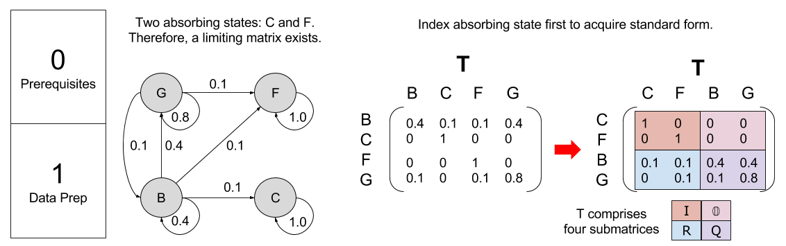
With T in standard form, we compute F = (I – Q)^-1 and T’.

Now that we know F and T’, we are in a position to answer questions with our data.

Thus, we are able to predict how Markov Chains will behave over the long run.

Takeaways

Markov Chains are convenient ways of expressing conditional probabilities graphically
But they require the Markov Property, that knowledge the present screens off any influence of the past.
We can compute expected locations by reasoning graphically.
However, it is simpler to compute expected locations by linear algebra techniques.
Linear algebra also enables us to discover what (some) Markov chains will approach, their limiting distribution.

Further Resources

To gain more intuition with linear algebra, see here.
To see Markov Chains applied to real-world situations, see here.
To see steady-state computations worked out in more detail, see here.

[Class] Bayesian Statistics

September 27, 2016September 27, 2016kevinbinz Leave a comment

So, over the summer I took it upon myself to teach a class on Bayesian Data Analysis, based on the following text,

This was a class put together for several coworkers, including members of our research team at Tableau. Here is a blurb summarizing course content:

Tableau provides various statistical methods, including primitives like Trend Lines (Regression). Our native solutions tend to use rely on Null Hypothesis Significance Testing, which are related to p-values, and a frequentist interpretation of probability. However, Bayesian Statistics is an alternative approach, that has been slowly been gaining traction in several fields.

This class introduced the technical details of Bayesian statistics. It ran July 19 – Sept 27, 2016 and used Doing Bayesian Data Analysis, Second Edition.

Weeks 1-3 will motivates the Bayesian approach to statistics.

Weeks 4-7 will give you tools to implement Bayes in R.

Weeks 8-10 will show how to use Bayesian alternatives to t-tests, regression, and ANOVA.

It was a great experience!

Week	Chapter	Date	Slides Available
1	Ch2: Intro to Bayesian Reasoning	July 19	Yes
2	Ch4: Intro to Probability Theory	July 26	Yes
3	Ch5: Intro to Bayes Theorem	Aug 2	No
4	Ch7: Markov Chain Monte Carlo (MCMC)	Aug 9	Yes
5	Ch9: Hierarchical Models	Aug 23	Yes
6	Ch11: Bayesianism vs Frequentism	Aug 30	No
7	Ch16: Bayesian t-test	Sept 6	No
8	Ch17: Bayesian linear regression	Sept 20	Yes
9	Ch19: Bayesian 1-way ANOVA	Sept 27	Yes

Your mileage may vary with the slides, of course. They work best in presentation mode – otherwise some of the transitions are a bit jumpy. I constructed these by myself, with lots of help from our textbook.

Glymphatic System: Why We Sleep

September 9, 2016August 29, 2017kevinbinz Leave a comment

Part Of: Demystifying Consciousness sequence
Content Summary: 1000 words, 10 min read

Introduction

At some point tonight, your movements will become lethargic, your eyes droop, and you will lose consciousness for eight hours.

This won’t be a one-time thing. You’ll spend twenty years of your life in this zombie state.

Together with reproduction and feeding, sleep appears to be one of the fundamental requirements of all vertebrates.

Why? Let’s find out!

Three Modes of Existence

An EEG takes electrical recordings of the scalp. If you use an EEG during sleep, you can distinguish different kinds of sleep:

There seem to be three modes of existence: wakeful consciousness, REM sleep, non-REM (NREM) sleep. These modes switch back and forth abruptly during a typical night’s sleep. Consider the following, a sleep architecture diagram:

sleep-stages-across-night-3

Chronobiological Influences

The rotation of the earth has profound implications on biological life. The temporal distribution of bodily functions is highly structured. Chronobiology studies biological rhythms.

Circadian rhythms are those that reset every 24 hours. The suprachiasmatic nucleus (SCN) drives your circadian clock. It is also a central hub of the hypothalamus, passing information to DMH to distribute to systems of feeding, stress, thermoregulation, and sleep:

sleep-hypothalamic-circadian-pathway-1

The pineal gland exists in nearly all vertebrates. It originally evolved with a third eye, which measured light intensity. However, mammals have long since lost their third eye, and instead splice retinal signals from the optic nerve to the hypothalamus, delivering light intensity data.

As long as there is light, the pineal gland is inert. However, with the onset of darkness, it produces melatonin. Melatonin thereby synchronizes the hypothalamus to the day-night cycle.

Ultradian rhythms are biological rhythms that reset more frequently than every 24 hours. Of these, the basic rest-activity cycle (BRAC) is most important. BRAC duration varies across species:

Cats exhibit a 20-minute rhythm in rate of responding. Likewise, it is been found that if one unobtrusively observes humans, they tend to show invigorated periods of facial grooming (eg touching the face, including nose picking) approximately every 90 minutes.

90 minute cycles have also been observed in heart rate, urine flow, eating, vigilance tasks, and tests for verbal and spatial intelligence. Importantly, these cycles need not start at the same time. Your peak time for verbal intelligence does not necessarily correspond with heightened face touching, but both will reset every ninety minutes.

Sleep is driven by the ventrolateral preoptic area (VLPO) of the hypothalamus. The VLPO incorporates the following systems:

circadian rhythms (sleep tends to occur at regular intervals);
ultradian rhythms (the REM-NREM cycle is 90min); and
melatonin production (sleep tends to be facilitated by darkness).

The Purpose of Sleep

Cellular metabolism uses adenosine triphosphate (ATP) to produce energy, which yields protein waste (metabolites) that float around outside of cells (interstitial space).

In the body, the lymphatic system is responsible for removing this waste. But in the brain, the blood-brain barrier (BBB) removes access to the lymphatic system. So, how does the brain remove metabolites?

Your brain does not rest against the base of your skull (that would destroy brain tissue). Instead, it is immersed in a fluid bath. This fluid is called cerebrospinal fluid (CSF)

In addition to surrounding the skull and inhabiting your ventricles, CSF also participates in the blood brain barrier. Specifically, CSF inhabits paravascular space (outside the blood vessel, but inside the astrocyte processes).

The cerebrospinal fluid flows between arteries & veins, creating a current that sweeps away metabolic waste. This is the glymphatic system:

In vein diameter, we see a tradeoff between metabolism (which uses blood, and produces waste) and glymphatics (which uses CSF, and removes waste).

During sleep, the brain consumes about 40% less energy. This means smaller vascular diameter, which in turn expands the paravascular channel. Therefore, we would predict that sleep would be favorable to glymphatic processes. And in 2013, it was confirmed that the glymphatic system is indeed 60% more effective during sleep.

Let me say that again. In 2013, we discovered why we sleep: to remove neural metabolites.

This discovery unifies two previously separate theories of sleep:

That sleep is metabolic (more difficult to catch food at night)
That sleep is restorative (that something is replenished by the act of sleep)

Homeostatic Influences

As we have seen, sleep urge involves more than simple neural oscillators. If a predator keeps an animal awake all night, that animal will feel an increased need to sleep. Excess metabolites induce a stronger urge to sleep.

A central organizing feature of the human body is the homeostatic setpoint, which regulates some quantity. For example, the brains of warm-blooded organisms represent and maintain blood temperature at a fixed value (in humans, 98.6 degrees Fahrenheit).

In this way, the part of the brain that regulates the body – the “hot loop” – can be conceived as a fairly elaborate kind of thermostat. And one such knob on this thermostat is sleep debt. But how does the brain represent sleep debt?

Adenosine is an inhibitory neuromodulator, ubiquitous in the vertebrate brain. Concentrations in the basal forebrain seem to represent sleep debt. Sleep deprived individuals have unusually high levels of adenosine, which is restored to normal levels only after a recovery sleep.

Along with biological oscillators, adenosine seems to induce sleep urgency. This is why caffeine works: it is an adenosine antagonist.

Importantly, adenosine is a metabolite. As adenosine triphosphate (ATP) is converted into cellular energy, adenosine (a byproduct of the reaction) is ejected from the cell into the interstitial space.

Adenosine not only measures time spent awake, but also directly represents the levels of toxins within your skull. Adenosine concentration is reduced during sleep because the glymphatic system removes it, along with other metabolites.

Adenosine thus provides another glimpse at the deep relationship between sleep and metabolism.

Takeaways

Mammals inhabit three modes of existence: wakeful consciousness, REM sleep, and non-REM sleep
Sleep is a consequence of metabolism: the brain uses sleep to remove metabolic waste via the glymphatic system.
Sleep is heavily influenced by circadian rhythms (reset every 24hr), ultradian rhythms (reset every 90min) and melatonin production.
Sleep is also influenced by adenosine, which is a more direct representation of ambient metabolites (and also, of course, sleep debt).

References

Saper et al (2005). Hypothalamic regulation of sleep and circadian rhythms
Kleitman (1982). Basic Rest-Activity Cycle-22 Years Later
Xie et al (2014). Sleep Drives Metabolite Clearance from the Adult Brain

The Lives of the Stars

July 27, 2016March 20, 2017kevinbinz Leave a comment

Part Of: Demystifying Physics sequence
Followup To: Deep Time
Content Summary: 1100 words, 11 min reading time.

Why does the Earth orbit a slow-burning hydrogen bomb? And why is the night sky illuminated with trillions of such explosions?

Let’s find out.

Preliminaries

Stars emit light. The most important characteristics of light are brightness and color. A Hertzsprung-Russell (HR) Diagram puts brightness on the x-axis, and color on the y-axis. In this way, a star can be represented by a single point.

What happens if you plot the location of all visible stars onto the same HR diagram? The result is rather striking:

Most stars seem to fit inside a continuous swathe known as the Main Sequence. Why?

As we will see, there are five stages in the stellar lifecycle:

Formation: Clouds congeal into protostars.
Dwarf Phase: Hydrogen begins to fuse.
Giant Phase: Hydrogen runs out, switch to helium fusion and beyond.
Fuel Crisis: nuclear fusion runs out of raw materials.
Termination: whatever remains of the star slowly becomes cold.

Stars spent 90% of their lives as dwarves. The radiation of dwarves vary continuously based on solar mass. This explains the Main Sequence.

As we will see, the five life-stages of the stars differ based on how big they are:

The Dynamics of Stars

Stars are born when hydrogen clouds begin to collapse in on themselves.

If gravity was the only force in play, all stars would quickly become black holes. But compressed gases develop high outward pressure. So there are a tension:

Phase 1: Protostars

Star formation begins when a molecular cloud begins to collapse into a dense core. As this core accretes mass, gravity’s pull intensifies. Soon, the site of collapse becomes a protostar.

Protostars are not yet hot enough to induce fusion. But the compression of gravity still makes these objects extremely hot. Once their radiation blows away surrounding clouds, the appear on what is called the stellar birthline of the HR diagram.

Small protostars are called T Tauri stars.
Large protostars are known as Herbig Ae/Be stars

As protostars mature, they become more hot and dense. On the HR diagram, their signatures will move from the stellar birthline towards the main sequence.

HR movement is not movement in space. “Travel” away from the stellar birthline means that protostars are growing hotter (left) but less bright (down).

Phase 2: Dwarves (Main Sequence)

The interior of the Sun is not homogenous. The closer to the center, the more extreme the climate. If the protostar is large enough, the core of the star will become so intense, that it will trigger nuclear fusion, releasing enormous amounts of energy. If space was not a vacuum, and the sound of the Sun could travel to Earth, its volume would equal that of a motorcycle.

Nuclear fusion { hydrogen → helium } depletes hydrogen, and creates helium. The helium core of the star expands, as hydrogen is depleted.

Small dwarf stars are called yellow dwarves.
Large dwarf stars are called blue dwarves.

Over 90% of a star’s lifetime is spent in this dwarf phase.

Stars are the crucible of matter. What does this mean?

The Primordial Era produced only hydrogen clouds, intermixed with helium. How is it possible for our bodies to be 65% oxygen? Hydrogen does not spontaneously become oxygen, after all.

With few exceptions, all naturally occurring substances were forged in the heart of stars. Nucleosynthesis describes how the raw material of the Big Bang was forged into the chemically diverse world of modernity. In the dwarf phase, we only see the construction of helium. We will soon see nuclear fusion carried much further.

We are literally made of starstuff.

Phase 3: Giants

Eventually, stars run out of hydrogen fuel. At this point, helium atoms are so hot that they start to fuse: { helium → carbon }. This new kind of fusion changes the thermal output of the star, which leaves the main sequence.

Helium-burning stars expand dramatically. For this reason, we call main-sequence stars dwarves, and post main-sequence stars giants.

Again we see a difference along solar mass:

Small stars in their giant phase are too small to combust carbon. These are red giants
Large giants can combust further elements. These are red supergiants

The interior of red supergiants, therefore, is shaped a bit like an onion, with each deeper layer “raising” the atomic number of its exterior. But why does this chain stop at iron?

Iron has the lowest mass per quark: fusing iron consumes energy, instead of creating it.

Small Stars: Fuel Crisis & Termination

Red giants eventually radiate away most of their mass. 😦 Thus, gravity slowly loses its hold on the star, and the outer shells are propelled outward by thermal pressure. This ejection of inert hydrogen is known as a planetary nebula.

The abandoned cores of a shell comprise white dwarves. Since these objects have no source of fuel, they slowly cool, resulting in down-right movement on a HR diagram:

Large Stars: Fuel Crisis & Termination

In contrast to smaller stars, supergiants die in fantastic ways. Their iron core is unstable, and will eventually explode in a supernova. Supernovae are no trifling matter. Their outputs are often brighter than their host galaxies (trillions of stars). If a nearby star in the Milky Way were to go supernova, it would obliterate the human race.

If the core survives the explosion, it becomes a neutron star. Neutron stars are rather dense. One teaspoon of its material would weigh more than ten Pyramids of Giza. Neutron stars are highly magnetic, and rotate quite swiftly: this is the root cause of quasars.

But sometimes the core will be even more dense. In this scenario, it will fully collapse into itself; ripping the fabric of spacetime to become a black hole. Black holes are a bit like predators; they “hunt” and “eat” other stars. At their center, most galaxies possess a supermassive black hole (SMBH). Our galaxy’s SMBH (Sagittarius A*) is fortunately 26,000 light-years away from Earth.

The Story of Our Sun

As we have seen, the universe is 13.8 billion years old, and stars began to form 13.4 billion years ago. We can categorize stars by birthday into three stellar populations.

The earliest stars were chemically simple because the universe contained nothing but hydrogen and helium. But as nucleosynthesis progressed, the universe began to accumulate more complex atoms. The second generation of stars had small amounts of metal. The last generation had substantial metal content.

Did you know that planets outnumber stars? There are about 200 billion stars in the Milky Way, and about 220 billion planets.

Planets are recent inventions. They are created only if a nebula sufficiently high metallic content. In that case, a protoplanetary disc will orbit the protostar, which will ultimately condense into extrastellar satellites.

As a recently-created star, born only 4.6 billion years ago, the Sun’s birthing nebula was sufficiently metallic to create such a disc. This disc eventually consolidated into our eight planets. The Sun is now in its second phase of life, a yellow dwarf. 5.5 billion years from now, it will – like so many of its brothers and sisters – start burning helium as a red giant.

Stellar Evolution- Our Sun (3)

Takeaways

Until next time.

An Introduction To Primate Societies

July 17, 2016February 15, 2019kevinbinz Leave a comment

Part Of: Anthropogeny sequence
Content Summary: 900 words, 9min read

Introduction

Primates are relatively young branch of the mammalian clade. Their anatomical characteristics are as follows:

Primates_ Anatomical Cladistics.png

There are three kinds of primate: prosimians (e.g., lemurs), monkeys (e.g., macaques), and apes (e.g., humans).

Primates are known for their large brains and a social lifestyle. Today, we will explore the dynamics of primate societies (defined as frequently interacting members of the same species).

There are three components of any society: the mating system (including sexual dynamics), the social organization (spatiotemporal organization of interaction), and the social structure (relational dynamics & social roles).

Sexual Dynamics

Because DNA is creepy, it programs bodies to make more copies of itself. Men and women are programmed with equally strong imperatives for gene replication (reproductive success). But female pregnancy powerfully breaks the symmetry:

Women spend more metabolic & temporal resources rearing children.
Women are certain that their offspring is their own, men can experience ambiguity.
A single woman can only produce one child at a time, a single man can impregnate many women concurrently.

It is because of pregnancy that males court females, and females choose males.

For females, paternal care is of tantamount importance: finding a mate willing to share the burden of raising a child. For males, fecundity is key.

We can see echoes of this asymmetry today. In all human cultures observed,

Women tend to be more jealous of emotional infidelity. Men have more violent reactions to sexual infidelity.
Women are statistically more interested in male social status and resources. Men pay comparatively more attention to physical beauty.

These gender differences arise as a response to the biological mechanism of pregnancy. These are contingent facts, nothing more. Species with male gestation, such as the seahorse, witness the reversal of such “gender roles”.

Four Mating Systems

From a logical perspective, there are exactly four possible mating systems.

Which mating system is biologically preferable? That depends on your gender:

Females benefit from polyandry, with multiple males available to raise offspring.
Males maximize their genetic impact with polygyny.

Most primates are polygynous. Why?

The answer is geographic. To survive, an animal must travel to surrounding land, locating flora or fauna to satisfy its metabolic budget. The amount of land it covers is known as its territory. The more fertile the land, the smaller the territory (less need to travel).

To mate with a female, a male will – of course – enter into that female’s territory. Thus, we can visualize each mating system from the lens of territory:

Mating systems are determined by female territory size.

If males can encompass the territories of multiple females, males will select polygyny (or, more rarely, promiscuity).
Otherwise, if females do not live in defensible groups, males will typically revert to monogamy (or, if females are sparse, polyandry).

In turn, female territory size is determined by environmental conditions. If the terrain is sparse, a female must travel further to sustain itself, and vice versa.

Our causal chain goes: plentiful land → smaller female territory size → polygyny. This is the Environmental Potential for Polygyny.

Three Social Organizations

The vast majority of primates are group living: they forage & sleep with bisexual groups of at least three adults. They spend most of their waking lives in the presence of one another. In other mammals, such group living is much less common.

Primates (e.g., humans) did not originally choose to live in groups because of their sociality. Predation risk induced group living. Only afterwards did primate brains adapt to this new lifestyle.

Some primates are exceptions to this rule. Two other, rarer, varieties of primate social organizations exist:

Some primates are solitary, foraging on their own. These species tend to be nocturnal. With less predation risk, individuals need not share territory.

Other primates live in pair bonds, a male-female pair. The attachment system is employed by infants to attach to their mothers: monogamous primates redeploy this system to support adult commitment. That said, primate monogamy only occurs when females live in an area that is difficult to defend.

We have seen 4 mating systems, and 3 social organizations. These are not independent:

Pair living and monogamy correlate. However, few primates live in such systems (thin line)
Group living and polygyny correlate: both are promoted by overlapping female territories. Most primates occupy this arrangement (thick line).

Structure: Dominance Hierarchy

When animals’ territory overlaps, they often compete (fight) for access to resources (food and reproductive access).

Fighting is accompanied with risk: the stronger animal could be unlucky, the weaker animal could lose their life. Similar to human warfare, both sides suffer less when the weaker side pre-emptively surrenders. The ability to objectively predict the outcome of a fight is therefore advantageous.

Suppose the need for fight-predictions is frequent, and do not often change (physical strength changes only slowly over an animal’s life). Instead of constantly assessing physical characteristics of your opponent, it is simpler to just remember who you thought was stronger last time.

This is the origin of the dominance hierarchy. The bread and butter of dominance hierarchies is status signaling. Dominant behaviors (e.g., snarling) evokes submissive behaviors (e.g., looking away).

Takeaways

We have explored three aspects of primate societies: mating system, social organization and social structure. Each of these is driven by external, ecological factors.

Primate Societies- Systemic View (4)

Primate niches typically feature high predation risk and fertile terrain. These promote female grouping, which in turn attracts males to live with them in groups, under a polygynous mating system.

Primates are unique for successfully living in groups throughout their long lifespan. To support this ability, primate brain volume increased, and came to provide increasingly sophisticated cognitive mechanisms & social structures.

We will explore the evolution of social structure next time. See you then!

References

Kappeler & Schaik, 2001: Evolution of Primate Social Systems.

An Introduction To Propriety Frames

July 8, 2016May 8, 2017kevinbinz 2 Comments

Part Of: Demystifying Ethics sequence
Content Summary: 1000 words, 10 min read

Preliminaries

Two important debates in philosophy of ethics go as follows:

Are our moral beliefs true, in some objective sense?
Is there some objective way to resolve moral disagreements, or claim moral progress? Or is it impossible to compare different moral systems?

For centuries, philosophers have wrestled with these issues. But the question of how minds construct morals in the first place, is underexplored.

Let me attempt to close the gap. In what follows, I describe probable mechanisms by which primates acquire intuitions about right and wrong.

We begin with a simple distinction:

Social attitudes (should / should not) are intuitions of socially appropriate behavior.
Moral attitudes (good / evil) are also judgments about behavior, but more associated with anger, inflexibility, and condemnation.

I submit that these two attitudes are weaved with the same fabric. To show this, I will address the following:

What are social attitudes?
Why do our social attitudes have the specific contents that they do?
Can moral attitudes be derived from social attitudes?

By the end, I hope you emerge with a clear understanding of how social and moral attitudes are constructed, shared, and used.

Propriety Frames

We are constantly immersed in highly structured interactions. The volume of these experiences can make social rules seem obvious: they become practically invisible. But by traveling to a sufficiently remote culture, or even spending time around a severely autistic person, we may begin to appreciate the sheer complexity of social norms.

Consider a typical evening at a fancy restaurant: how many social rules can you think of? Here are a few examples of “breaking the rules”:

The waiter states he is not in the mood to take your order.
Several guests are engaged in a foodfight.
The food is dumped directly on the table.
On taking a bite, you realize that your meal is actually plastic: an artistic creation designed purely for visual effect.
An extravagant item on the menu is free of charge.
Instead of payment, the manager comes out to request that you wait tables next weekend.

This list could go on for many pages. It may take a while to generate such a list, but you could immediately recognize if any one of thousands of such “rule violations” occur. This suggests that your brain contains vast amounts of social information. But how is this information acquired? How is it retained?

In social psychology, schema or frames are often employed as useful ways to bundle collections of facts. Frames can nest within one another. For example, our restaurant expectations are a propriety frame with three constituents: Host-Guest, Eating, and Place Of Business. Surprises {1, 2} are violations of the host-guest frame, {3, 4} countermand the eating frame, {5, 6} negate the place of business frame.

Propriety Frames- Restaurant Example (3)

Propriety frames store knowledge of socially appropriate behaviors, just as semantic memory retains factual knowledge. Whereas semantic memory can be communicated in simple sentences, norms are communicated in larger narrative structure. Norm synchronization plays a large role in the human delight in stories.

This simple model provides great insight into common social experiences. When you watch a mother instruct her son to not to yell in the store, you are watching the child install an update to his Shopping frame. When a family exchanges gossip around a campfire, they are synchronizing their frames.

Frame Attractors

How are propriety frames represented within the brain?

A clue comes from semantic representation. It seems that the brain has not one, but three languages through which it encodes facts:

Prototypes are bodies of statistical knowledge about a category. A Dog prototype could store properties that are diagnostic of the class of dogs.
Exemplars are bodies of knowledge about individual members of a category. An Dog exemplar would be e.g., of the last dog you saw.
Theories are bodies of causal, functional, and nomological knowledge about categories. A Dog theory would consist of such knowledge.

A frame doesn’t need to be huge lists of rules. It is more flexibly encoded as a prototype: a statistical “center of gravity” which represents a behavioral ideal. This prototype need not correspond to observed behavior, just as you can understand triangles without encountering a geometrically perfect triangle.

Let us imagine behavior space, where complex behaviors are compressed into dots at a single location. In this picture, our propriety frame is just another point.

On this metaphor, violations of social rules are simple vector calculations, from observed behavior to that person’s moral standard. A propriety frame is an attractor which compares all observed behavior to itself.

If propriety frames were simple lists of rules, it would be hard to explain why some violations appear worse than others. By using prototypes, the brain preserves severity information. The larger the vector, the more salient the violation.

A Physical Mechanism

Recall that brains are organized into two perception-action loops:

The Somatic Loop processes the world: it maps perception → action
The Visceral Loop processes the body: it maps feeling → motivation.

Semantic memory is extremely perceptual in nature. Sense data travels from skin, eyes, ears, and coalesce into perceptual object files such as Dog.

In our discussion so far, we have described the role of frames in social appraisal. However, propriety frames serve two distinct functions:

Action: The Restaurant Frame produces motor command signals, which travel towards primary motor cortex, then down the brainstem.
Appraisal: The Restaurant Frame compares its behavioral ideal to observed behavior. The output of this comparison is then delivered to our limbic systems. This is why inappropriate behavior can cause an emotional reaction, and also motivate us to act (e.g., to exchange awkward looks).

Propriety Frames- Two Loops (5)

Hume once remarked that it is hard to see how descriptive science can relate to prescriptive attitudes. However, the solution to this is-ought gap has become clear. Cognitive science can bridge the gap by describing how propriety frames drive our motivational apparati.

Summary

The brain contains many knowledge systems. Propriety frames are just another such system.

Consider the sentence “So, Jane and I visited this restaurant, and the waiter says to me …”. As your brain’s Visual Word Form Area (VWFA) processes the symbols within that sentence, your brain will automatically retrieve information about the people, nouns, and social conventions relevant to that sentence. This information is then brought into the Global Workspace of conscious attention.

Propriety frames are simply another service provided by our wonderful brains. 🙂 Next time, we will explore how this system comes to develop specific judgments about behavior.

Until next time.

The Birth of the Universe

June 26, 2016June 15, 2019kevinbinz Leave a comment

Part Of: Demystifying Physics sequence
Content Summary: 1200 words, 12 min reading time.

Our lifespan is 80 years. Our consciousness refreshes every 300 milliseconds. Timespans beyond these, human brains are not well-equipped to conceive. Nevertheless, to learn the origin story of the universe, we must stare into the abyss of deep time.

Where do we come from?

Poets, philosophers and theologians have explored this question for millennia, in part seeking to ascribe meaning to the cosmos. Only recently have we discovered a literal answer, which constrains and complements our narratives.

Here are the facts.

Particle Physics

The universe is built from fermions and bosons.

Fermions are the bedrock of matter, the “meat” in our particle soup. They come in two flavors: quarks and leptons. You’ve heard of antimatter, yes? This term refers to antiquarks and antileptons.

In contrast, bosons are force carriers; the “broth” of the soup. They mediate the four fundamental forces: gravity, the strong force (which holds atoms together), the weak force (radioactivity), and electromagnetism (literally everything else).

Here are the most significant species of particles:

Protons & neutrons are not elementary particles. They are coalitions! Gluons combine quarks into groups called hadrons. When hadrons contain three quarks, they are called baryons.

Hydrogen is one electron orbiting one proton; that is, one lepton orbiting three quarks!

The Primordial Era

13.8 billion years ago, the Big Bang happened. At that moment, a gravitational singularity (the primeval atom) exploded, and became the basis of all matter, energy, space and time.

What happened before the Big Bang? This question is incoherent: it reduces to “what happened before time existed”?
What happened after the Big Bang? To answer this, let us divide time into eight segments.

1. Planck Epoch (0 → 10^-43 sec). The climate of this period of history is so intense, known laws of physics break down. We suspect that gravity merges with the other forces, but we do not yet possess a theory of quantum gravity. Only with such a Theory of Everything can we hope to better understand what caused the Big Bang.

2. Grand Unification Epoch (10^-43 → 10^-36 sec). Science recovers its ability to describe nature during this epoch. The Strong, Weak, and Electromagnetic Forces exist as a single entity: the electronuclear force. The universe is expanding, but it is still a small, hot ball of plasma. Physical characteristics like mass, charge, etc are completely meaningless.

3. Inflationary Epoch (10^-36 → 10^-32 sec). Next, the mysterious phenomenon of cosmic inflation obtained. The fabric of spacetime explodes at a rate that far, far exceeds the speed of light. The volume of the universe expands at least seventy-eight orders of magnitude (10⁷⁸ times bigger).

Few people realize the implications of such an overpowered process. Have you heard the phrase observable universe? Buried within this phrase is the implication of unobservable universes. You don’t need to wander into QM interpretations to encounter Many Worlds. We already know that there are myriad universes that we can never access: inflation simply pushed them beyond any distance our radio signals could traverse.

4. Electroweak Epoch (10^-32 → 10^-12 sec). At the end of this epoch, the universe has cooled enough for the Strong force to dissociate from the Electroweak force. Quarks, antiquarks, and gluons dominate the cosmos.

5. Quark Epoch (10^-12 → 10^-6 sec). Despite the newly independent Strong force, quarks are unable to combine. Ambient temperature is too hot, preventing nuclear fusion.

6, 7. Hadron Epoch, and Lepton Epoch (10^-6 → 10 sec) . Things have finally cooled enough for quarks and antiquarks to combine! The universe fills with hadrons (e.g., protons) and anti-hadrons (e.g., anti-protons).

In this era, matter slightly outnumbered antimatter, for reasons we don’t yet understand.

Antimatter was suppressed during these epochs. At the end of the Hadron Epoch, most hadrons and anti-hadrons experience annihilation reactions. The few survivors were matter: this is baryogenesis (baryons are a species of hadron).

In the subsequent Lepton Epoch, leptons and anti-leptons (e.g., electrons and anti-electrons) also annihilate one another en masse. Antimatter was again underrepresented in the survivors: this is leptogenesis.

8. Photon Epoch (10 sec → 380,000 years). 10 seconds after the big bang, and photons dominate the universe. Protons and electrons (hadrons and leptons) exist, but are unable to come together due to high temperatures. The free electrons scatter light: photon travel is randomized by collisions with free electrons, in a process known as Compton scattering.

As the fabric of spacetime continues to expand, two other things happen:

Recombination: Temperatures drop to a point where electrons and protons could come together to form hydrogen atoms!
Rise of the Fermions: The expansion of space stretches photon wavelength, decreasing its total energy content. Fermions, whose populations had been decimated in the destruction of antimatter (c.f. baryogenesis and leptogenesis), reclaim the title as the most energetic substance in the universe.

The eventual result was photon decoupling. Temperature finally permits light could travel freely. The universe becomes transparent.

You’ve probably heard that it takes light from the Sun eight minutes to reach Earth. If the Sun suddenly disappeared, we would only learn that fact eight minutes later. Similarly, if a star 40,000 light-years away suddenly explodes in a supernova, we must wait until 42,016 AD to learn about that. Starlight is a form of time-travel.

What are the oldest photons we can see? How far back into our past can we peer?

Well, we can see galaxies being formed 200 million years after the Big Bang. And we can peer back farther still. We can directly see light emitted the moment the universe became transparent; this is the Cosmic Microwave Background (CMB).

Why is the CMB not smooth? The ripples are microscopic phenomena writ large: inflation exploded quantum fluctuations on a cosmic scale…

Deep Time- Cosmic Background Radiation (1)

Some of the static in TV antenna is caused by the CMB. You can literally see evidence of the Big Bang with your own eyes.

Structure Formation

Photon decoupling has ensured that light can travel freely in a sea of hydrogen. However, there were no stars at this point: the CMB is the only light source. This is the Dark Age of the universe, a time before stars.

Why is so much of space a vacuum?

In the Inflationary Epoch, inflation etched ripples into the energy distribution of the cosmos. Gravity accentuates this heterogeneity by pulling matter together. Space is mostly empty because particles like to spend time together.

Gravity appears to operate at three different spatial frequencies.

Very large clumps of hydrogen become superclusters.
Within every supercluster, there are billions of smaller clumps called galaxies.
Galaxies in turn comprise billions of smaller assemblies: stars and solar systems

The origin of all things is the hydrogen cloud, and gravitational attraction.

Takeaways

There are two kinds of particles in the universe: fermions (“matter particles”) and bosons (“force particles”)
The Big Bang happened 13.8 billion years ago. The early universe was hot, and expanded quickly.
Three important events in occur in the first second of the universe
- Cosmic Inflation: the fabric of the universe stretched much faster than the speed of light, creating unobservable universes.
- Force Differentiation: the four forces (gravity, strong, weak, electromagnetic) separated from one another
- Fermion Asymmetry: antimatter was preferentially annihilated

Afterwards, the universe was replete with clouds of hydrogen. Gravity pulled these together to form stars, galaxies, and superclusters.

The Three Stream Hypothesis

June 6, 2016March 23, 2017kevinbinz 3 Comments

Part Of: Neuroanatomy sequence
Content Summary: 1000 words, 10 min read

Blindsight

Have you heard of blindsight before?

This man has no conscious experience of vision. And yet, he can avoid obstacles while walking! Blindsight is not a trick, and hundreds of cases are documented. How can a person see, but not know that he sees?

To answer, we turn to the brain.

Two Visual Streams

Recall our concept of flat map. Cortex is like a sheet: its wrinkles can be stretched flat.

Green areas are primary areas: landing sites of different sensorimotor modalities. The visual primary area is V1, somatosensory touch is S1, muscles is M1.

Visual information is pumped from the retina to V1. From there, the Dual Stream Hypothesis suggests that it follows two distinct pathways:

The traditional graphic illustrates how visual information passes up into the dorsal stream, and down into the ventral stream.

Things become more clear with a flat map (right). Consider the phenomenon of hand-eye coordination involved in, e.g., playing table tennis. Moving the paddle to return a serve require close collaboration between visual information (about the ball) and motor information (from the hand). Here, it seems clear that hand-eye coordination is provided by the dorsal stream, which comprises the shortest distance between V1 and M1.

Blindsight patients have damage to V1. They are not conscious of visual experiences, yet their ability to maneuver obstacles suggests that their hand-eye coordination (Dorsal stream) is still intact. How can this be?

Well, the optic nerve also passes information directly to the dorsal stream. While the Ventral Stream of V1-damaged blindsight patients receives no information, the Dorsal Stream remains functional.

Inspired by these blindsight patients, Milner & Goodale gave these streams nicknames.

The Dorsal How Stream performs hand-eye coordination
The Ventral What Stream produces conscious perception.

Our subjective experience of unitary vision is wrong! If you step back, though, it makes perfect sense for natural selection to carve out two flavors of vision, each with different purposes. Action-based vision needs to happen quickly; perceptual-based vision is more analytical and doesn’t have the same speed requirements.

Tension In The Dorsal Stream

The Dual Stream Hypothesis is grounded in strong neuroscientific and behavioral evidence. It also has enjoyed consensus support from neuroscientists for nearly two decades. However, there are also some notes of tension.

Conceptual tension to a researcher is blood to a shark.

Did you know there are actually two versions of the Dual Stream Hypotheses? Goodale & Milner’s 1992 version (explored above) is the most well-known, but in 1982 Mishkin et al also proposed a Dual Stream model, based on monkey lesion studies. Both accounts agree about the Ventral What Stream. But Mishkin’s model gives a spatial processing role to the Dorsal Stream (“Where”). Why should these research traditions view the Dorsal Stream so differently? Note well such cases of functional tension.

Let me advance two observations that are unique to myself.

First, consider the width (angular spread) of the two streams. In the above flat map, notice how much wider the Dorsal Stream is than the Ventral Stream (nearly three times wider!). How can the Dorsal Stream be so wide, yet retain functional coherence? This is structural tension. While such hints are less damning, they destabilize our already queasy relationship with the Dorsal Stream.

Second, it is curious that roughly ⅓ of the cortical area around V1 are simply not recruited in the Dual Stream Hypothesis. Surely such regions (e.g., Lingual and Cuneus cortex) have some role in the processing of visual information. Could these medial regions comprise a fourth stream?

Call this the Medial Stream Conjecture. The medial stream seems to project directly the hippocampus. I suspect that in five years, we shall speak of the Medial Experiential Stream, which supports autobiographical memory.

The Lateral Stream: Healing The Divide

A parable of three disciplines:

The cognitive psychologist speaks the language of function. How does the mind create behavior?
The neurophysiologist speaks the language of structure. How do anatomical minutiae participate in neural circuitry?
The cognitive neuroscientist serves as translator. She pursues structure-function maps; the connective tissue between biology and information processing.

Sometimes these maps go awry, and must be repaired. The Dorsal Stream → { What or Where } map is such a case.

Several researchers have proposed that the Dorsal Stream be split into two separate streams (e.g., Rizzolatti & Matelli, 2003). Call this the Three Stream Hypothesis. The “true” Dorsal Stream is more narrow, and retains its How functionality. However, the remaining cortical surface is now called the Lateral Stream, which performs spatial processing (Where).

Milner’s Dorsal How Stream was much too wide. Conversely, Mishkin’s “Dorsal” Where Stream is actually located more laterally.

The Lateral and Dorsal streams both connect posterior parietal to premotor cortex. Two decades ago, these areas were largely referred to by name (“the premotor cortex does X”). Modern treatments, however, parcellate these regions at a much finer granularity. This also helps explain how Milner and Mishkin conflated the streams.

Integrating Audition

Originally, the dual stream hypothesis was viewed as only relevant to vision. However, lately there has been an influx of interest in auditory streams. The seminal paper is Hickok & Poeppel (2007), The cortical organization of speech processing. It proposes two streams:

The antero-ventral stream (green, left) performs auditory classification, and assists in speech comprehension.
The postero-dorsal stream, (red, right) in contrast, is not bilaterally symmetric.
1. The postero-dorsal stream in the right hemisphere localizes auditory stimuli both spatially and temporally.
2. The postero-dorsal stream in the left hemisphere performs speech production.

The auditory stream model integrates cleanly with the Three Stream Hypothesis. The auditory antero-ventral stream shares real estate with the Ventral stream. The auditory postero-dorsal stream overlaps the Lateral stream.

Why is “deafhearing” (an auditory version of blindsight) impossible? Because ear-hand coordination is not a thing. Auditory information simply does not participate in the unconscious Dorsal stream.

Summing Up

The Three Stream Hypothesis describes how auditory and visual information are carried as far as the prefrontal cortex. We may carve each stream into three discrete phases:

Finally, we can also visualize these same relationships more abstractly, as follows:

Until next time.

Perceptual Objects: Implications for AI and Philosophy

June 4, 2016June 5, 2016kevinbinz Leave a comment

Part Of: Object sequence
Followup To: The Language of Consciousness

Introduction

Objects are distributed networks: their resident features are computed in myriad locations across cortex.

Objects are an extremely rich concept, at the intersection of several disciplines. Given their explanatory fecundity, they will undoubtedly play an important role in the future of philosophy. Let me gesture at a few conversations where this is especially true.

Logical vs Statistical Inference

There have been two distinct waves of Artificial Intelligence research. The first was inspired by symbolism, which basically held the brain as maneuvering within a formal system of logic (recall that logic is computation). The approach fell out of favor after the discovery of the frame problem. In the 1980s, a new approach to AI rose from the ashes, this time fueled by connectionism and powerful methods of probabilistic inference.

These approaches comprise the Great AI Schism:

Each programme has its own unique strength

The logical approach excels at modeling complexity within its environment
The statistical approach excels at representing uncertainty within its beliefs.

There is reason to believe that AI will accelerate significantly once it discovers how to weld these approaches together. But the solution has not yet been discovered.

Object files may provide insight. You see, the human mind seems able to perform two kinds of mental operations:

Slow, serial, conscious inference (e.g., long division)
Fast, parallel, pre-conscious inference (e.g., finding a red hat in a crowd)

The behavioral evidence for such “modes of thought” has motivated dual process theory. Don’t these modes remind you of our statistical vs logical divide?

Objects are the middleware that straddles the logical-statistical divide. Understanding their mechanics may at last heal the AI Schism.

Problem Of Intentionality

One of the most protracted philosophical objections to the cognitive revolution goes as follows:

Computers are formal systems which manipulate abstract symbols (e.g., program variables). CPUs play games with these variables, but they have don’t participate in the meaning of these symbols. For example, a weather program will update the bits of EXPECTED_TEMP, without access to the physical interpretation of such a symbol.

Call this the problem of intentionality. For another example, we turn to Searle’s Chinese Room thought experiment:

Imagine an enormously sophisticated rulebook, billions of lines long, with the following format:

IF Chinese character X is slipped under the door THEN output Chinese Y.

Imagine John, an English speaker, enters the room containing this rulebook, and closes the door. His bilingual friend Wei slips Chinese sentences under the door. Following these rules in the book, John pushes characters under the door. To Wei’s astonishment, these characters compose Chinese sentences. What’s more, Wei experience a lively conversation in Chinese.

Does anyone understand what Wei is saying? Not John. He doesn’t speak Chinese! And it is absurd to attribute understanding to the pages of the rulebook. The room is behaving like a human, but does not understand.

Therefore, Searle claims, even if AI could pass the Turing Test, it would never understand in the same sense that Wei understands.

Object construction is the road by which philosophers will solve intentionality. As Harnad puts it in his excellent 1990 paper:

Symbolic representations must be grounded bottom-up in nonsymbolic representations of two kinds:

“iconic representations” , which are analogs of the proximal sensory projections of distal objects and events, and

“categorical representations”, which are learned and innate feature-detectors that pick out the invariant features of object and event categories from their sensory projections.

In other words, the brain performs symbol grounding: translating the symbol RED into non-symbolic imagery! Once we understand how objects cash out in sensorimotor systems, we will have explained how the brain injects semantic meaning into its knowledge systems. Why should such a mechanism be limited to meat. 🙂

Cognitive Epistemology

Philosophers concern themselves, among other things, with the definition of truth. The most widely accepted definition, the correspondence theory of truth goes like this:

The truth or falsity of a statement is determined by how well its contents correspond to the world.

This philosophical frame coheres well with the cognitive notion of representation. A representation can fail to reflect the structure of reality: the map is not the territory. But some representations can correspond to reality, in a strict, mathematical sense.

Plantinga’s Evolutionary Argument Against Naturalism (EAAN) discusses the relationship between naturalism, biological fitness, and knowledge. If natural selection is the driver for organism design, how do we know that our brains are constructing truth? That our maps really do correspond with reality?

Adaptive behavior, after all, does not require true beliefs:

Perhaps Paul very much likes the idea of being eaten, but when he sees a tiger, always runs off looking for a better prospect, because he thinks it unlikely the tiger he sees will eat him. This will get his body parts in the right place so far as survival is concerned, without involving much by way of true belief.

The question reduces to, is adaptive behavior orthogonal to knowledge?

As I like to say, “epistemology without psychophysics is dead”. If you want to understand the trustworthiness of human knowledge acquisition systems, you cannot responsibly ignore the brain. Empirically literate epistemology is, regrettably, still in its infancy. However, cognitive epistemology cannot proclaim victory at early perceptual areas. We want to know whether we can retain this sense of trust from the retina to beliefs more accessible to conscious awareness (i.e., beliefs grounded in objects).

Until next time.

Feature Binding: The Language of Consciousness

June 4, 2016May 8, 2017kevinbinz Leave a comment

Part Of: Object sequence
Content Summary: 400 words, 4 min read

Binding Via Phase Locking

As we have seen, objects are distributed networks: their resident features are computed in myriad locations across cortex.

The binding problem is: how do these distributed networks cohere? How does geographic division become logical unity?

Object binding seems to be accomplished via phase locking. By some unknown mechanism, firing patterns from disparate features synchronize, such that they all strike consumer processes simultaneously. By this temporal mechanism, objects increase their “firing power” while not needing to amplify their component signals.

Phase locking can be observed in the electrical rhythm of the brain, as measured by the electroencephalogram (EEG). Phase locking is only observed during the wakeful state, disappearing with the onset of Slow Wave Sleep (SWS).

We hypothesize that phase locking is necessary for object creation; that it is the solution to the binding problem. But phase locking only occurs during wakefulness. This suggests that object creation and consciousness are closely interrelated processes.

Let us conjecture that objects are the language of consciousness. They are the Song of Cortex.

This hypothesis provides explanatory firepower. We may now dissolve two Gordian knots.

The Unconscious Dorsal Stream

Remember blindsight? We explored blindsight in The Three Stream Hypothesis: blindsight patients have visual information accessible to the Dorsal Stream, but not the Lateral nor Ventral Stream.

But why should the Dorsal Stream be uniquely non-conscious? This is one of GWTs big open questions, as acknowledges by Baars in Global Workspace Dynamics, 2013. But we have made two conceptual moves that Baars has not:

Objects are the language of consciousness
Objects are created across by a ventral Classifer and a lateral Localizer engine (see Dual Engine Hypothesis, here).

The Dorsal Stream is unconscious because it does not participate in object construction.

Chunking

In the working memory literature, chunking refers to the ability to retain more information via drawing creative boundaries around information. Suppose I were to verbally recite the following phone numbers:

“2-0-6-5-5-5-1-2-2-0”
“206-555-220”

Both sounds encode the same information, but you could remember the latter more easily. Why?

It is widely acknowledged that the contents of working memory are available to consciousness. If working memory is the Global Workspace, then we would expect that chunks are objects. And indeed, our conjecture does successfully explain chunking:

In the above example, we retain the chunked version better because it requires the activation of only three objects (206, 555, 1220), rather than ten, single-digit objects.

Takeaways

Evidence of phase locking suggests that objects are the language of consciousness:
Objects are created by two engines: a Localizer and a Classifier. The Dorsal stream contains neither engine, and is thus non-conscious.
Objects explain working memory results such as chunking.

Fewer Lacunae

Distilled, Integrative Research

Author kevinbinz

An Introduction To Markov Chains

[Class] Bayesian Statistics

Glymphatic System: Why We Sleep

The Lives of the Stars

An Introduction To Primate Societies

An Introduction To Propriety Frames

The Birth of the Universe

The Three Stream Hypothesis

Perceptual Objects: Implications for AI and Philosophy

Feature Binding: The Language of Consciousness