An Introduction to Geometric Group Theory

November 7, 2017November 9, 2017kevinbinz 1 Comment

Part Of: Algebra sequence
Followup To: An Introduction to Abstract Algebra
Content Summary: 1500 words, 15 min read

An Example Using Modular Addition

Last time, we saw algebraic structures whose underlying sets were infinitely large (e.g., the real numbers $\mathbb{R}$ ). Are finite groups possible?

Consider the structure $( \left\{ 0, 1, 2, 3 \right\}, +)$ . Is it a group? No, it isn’t even a magma: $2 + 3 \not\in \left\{ 0, 1, 2, 3 \right\}$ ! Is there a different operation that would produce closure?

Modular arithmetic is the mathematics of clocks. Clocks “loop around” after 12 hours. We can use modulo-4 arithmetic, or $+_{4}$ , on $\left\{ 0, 1, 2, 3 \right\}$ . For example, $2 +_{4} 3 = 1$ .

To check for closure, we need to add all pairs of numbers together, and verify that each sum has not left the original set. This is possible with the help of a Cayley table. You may remember these as elementary school multiplication tables 😛 .

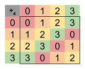
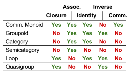
Geometrical Group Theory_ C4 Cayley Table Modular Arithmetic

By inspecting this table, we can classify $Z_4 = ( \left\{ 0, 1, 2, 3 \right\} ), +_{4})$ .

Does it have closure? Yes. Every element in the table is a member of the original set.
Does it have associativity? Yes. (This cannot be determined by the table alone, but is true on inspection).
Does it have identity? Yes. The rows and columns associated with 0 express all elements of the set.
Does it have inverse? Yes. The identity element appears in every row and every column.
Does it have commutativity? Yes. The table is symmetric about the diagonal.

Therefore, $Z_4$ is an abelian group.

An Example Using Roots of Unity

Definition 1. A group is said to be order $n$ if its underlying set has cardinality $n$ .

So $Z_4$ is order 4. What other order-4 structures exist?

Consider the equation $i^4 = -1$ . Its solutions, or roots, is the set $\left\{ 1, i, -1, -i \right\}$ . This set is called the fourth roots of unity.

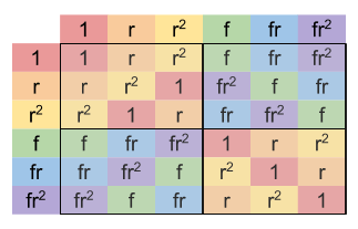
So what is the Cayley table of this set under multiplication $R_{4} = ( \left\{ 1, i, -1, -i \right\}, *)$ ? In the following table, recall that $i = \sqrt{-1}$ , thus $i^2 = (sqrt{-1})^2 = -1$ .

Geometric Group Theory_ C4 Cayley Table Roots of Unity (1)

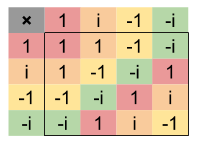
Something funny is going on. This table (and its colors) are patterned identically to 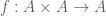$Z_4$ ! Recall that a binary operation is just a function $f : A \times A \rightarrow A$ . Let’s compare the function maps of our two groups:

Cyclic Groups_ Binary Operation as Function (2)

These two groups for structurally identical: two sides of the same coin. In other words, they are isomorphic, we write $Z_{4} \cong R_{4}$ . Let us call this single structure $C_4$ .

But why are these examples of modular arithmetic and complex numbers equivalent?

One answer involves an appeal to rotational symmetry. Modular arithmetic is the mathematics of clocks: the hands of the clock rotating around in a circle. Likewise, if the reals are a number line, complex numbers are most naturally viewed as rotation on a number plane.

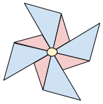
This rotation interpretation is not an accident. It helps use more easily spot other instances of $C_4$ . Consider, for instance, the following shape.

Geometric Group Theory_ Rotational Symmetry Object

On this shape, the group of rotations that produce symmetry is $W_4 = (\left\{ 0, 90, 180, 270 \right\}, \text{rotate})$ . Inspection reveals that this, too, is isomorphic to $C_{4}$ !

Towards The Presentation Formalism

We describe $C_3$ as a cyclic group, for reasons that will become clear later.

Theorem 2. For every cyclic group $C_n$ , there exists some generator $g$ in its underlying set such that every other set element can be constructed by that generator.

Definition 3. When a generator has been identified, we can express a group’s underlying set with generator-dependent names. Two notation are commonly used in practice:

In multiplicative notation, the elements are renamed $\left\{ e, r, r^2, r^3 \right\}$ , where r is any generator.
Similarly, in additive notation, the elements become $\left\{ e, r, 2r, 3r \right\}$ .

Geometric Group Theory_ Multiplicative and Additive Notation (1)

These two notation styles are interchangeable, and a matter of taste. In my experience, most mathematicians prefer multiplicative notation.

What generators exist in $C_4$ ? Let’s look at our three instantiations of this group:

In modular arithmetic, you can recreate all numbers by $0 + 1 + 1 + \ldots$ . But you can also recreate them by $0 + 3 + 3 + \ldots$ .
In complex numbers, you can visit all numbers by multiplying by $i$ , or multiplying by $-i$ . Only $-1$ fails to be a generator.
In our rotation symmetry shape, two generators exist: clockwise $90 \circ$ rotation, and counterclockwise $90 \circ$ rotation.

For now, let’s rename all elements of $C_{4}$ to be $C_4 = (\left\{ 0, 1, 2, 3 \right\}, +) = \langle 1 \rangle = \langle 3 \rangle$ .

Okay. But why is $2$ not a generator in $C_4$ ?

Theorem 4. For finite groups of order $n$ , each generator must be coprime to $n$ . That is, their greatest common divisor $\text{gcd}(g, n) = 1$ .

$2$ not a generator in $C_4$ because it is a divisor of $| \left\{ 0, 1, 2, 3 \right\} | = 4$ .
What are the generators in $C_5$ ? All non-identity elements: $C_{5} = \langle 1 \rangle = \langle 2 \rangle = \langle 3 \rangle = \langle 4 \rangle$ .
What are the generators in $C_6$ ? Only 1 and 5: $C_{5} = \langle 1 \rangle = \langle 5 \rangle$ .

We just spent a lot of words discussing generators. But why do they matter?

Generators are useful because they allow us to discover the “essence” of a group. For example, the Rubik’s cube has $5.19 \times 10^{20}$ configurations. It would take a long time just writing down such a group. But it has only six generators (one for a $90 \circ$ rotation along each of its faces) which makes its presentation extremely simple.

Another way to think about it is, finding generators is a little bit like identifying a basis in linear algebra.

Towards Cayley Diagrams

Definition 5. We are used to specifying groups as set-operator pairs. A presentation is an generator-oriented way to specify the structure of a group. A relator is defined as constraints that apply to generators. A presentation is written $\langle \text{generators} \mid \text{relators} \rangle$

In multiplicative notation: $C_4 = \langle r \mid r^3 = e \rangle$ .
In additive notation: $C_4 = \langle r \mid 3r = e \rangle$ .

The $= e$ suffix is often left implicit from presentations (e.g., $C_4 = \langle r \mid r^n \rangle$ ) for the sake of concision.

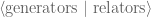
Definition 6. A Cayley diagram is used to visualize the structure specified by the presentation. Arrow color represents the generator being followed.

Note that Cayley diagrams can be invariant to your particular choice of generator:

Geometric Group Theory_ Cayley Diagram (1)

The shape of the Cayley diagram explains why $C_3$ is called a cyclic group, by the way!

With these tools in hand, let’s turn to more complex group structures.

Dihedral Groups

Cyclic groups have rotational symmetry. Dihedral groups have both rotational and reflectional symmetry. The dihedral group that describes the symmetries of a regular n-gon is written $D_{n}$ . Let us consider the “triangle group” $D_{3}$ , generated by a clockwise $120\circ$ rotation $r$ and a horizontal flip $f$ .

With triangles, we know that three rotations returns to the identity $r^3 = e$ . Similarly, two flips returns to the identity $f^2 = e$ . Is there some combination of rotations and flips that are equivalent to one another? Yes. Consider the following equality:

Geometric Group Theory_ Rotation vs Reflection Equivalence (2)

Analogously, it is also true that $rf = fr^2$ .

Definition 7. Some collection of elements is a generating set if combinations amongst only those elements recreates the entire group.

Cyclic groups distinguish themselves by having only one element in their generating set. Dihedral groups require two generators.

We can write each dihedral group element based on how it was constructed by the generators:

$D_n = \left\{ e, r, r^2, \ldots, r^n-1, f, rf, r^2f, \ldots, r^{n-1}f \right\}$

Alternatively, we can instead just write the presentation of the group:

$D_{3} = \langle r, f \mid r^3 = 1, f^2 = 1, r^2f = fr, rf = fr^2 \rangle$ .

We can visualize this presentation directly, or as a more abstract Cayley graph:

Geometric Group Theory_ Dihedral Groups Intro (3)

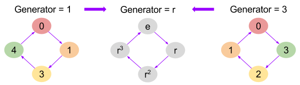
The Cayley table for this dihedral group is:

Geometrical Group Theory- Dihedral Cayley Table

This shows that $D_3$ is not abelian: its multiplication table is not symmetric about the diagonal.

By looking at the color groupings, one might suspect it is possible to summarize this $6 \times 6$ table with a $2 \times 2$ table. We will explore this intuition further, when we discuss quotients.

Until next time.

Wrapping Up

Takeaways:

Finite groups can be analyzed with Cayley tables (aka multiplication tables).
The same group can have more than one set-operation expressions (e.g., modular arithmetic vs. roots of unity vs. rotational symmetry).
Generators, elements from which the rest of the set can be generated, are a useful way to think about groups.
Group presentation is an alternate way to describing group structure. We can represent presentation visually with the help of a Cayley diagram.
Cyclic groups (e.g., $C_3$ ) have one generator; whereas dihedral groups (e.g., $D_3$ ) have two.

Related Resources

This post is based on Professor Macaulay’s Visual Group Theory lectures, which in turn is based on Nathan Carter’s eponymous textbook.
Related to this style of teaching group theory are Dana Ernst’s lecture notes.
If you want to see explore finite groups with software, Group Explorer is excellent.
For a more traditional approach to the subject, these Harvard lectures are a good resource.

An Introduction to Abstract Algebra

October 30, 2017November 12, 2017kevinbinz Leave a comment

Part Of: Algebra sequence
Content Summary: 1200 words, 12 min read

A Brief Prelude

Recall that a set is a collection of distinct objects, and a function $f: A \rightarrow B$ is a mapping from the elements of one set to another. Further, in number theory we can express numbers as infinite sets:

The natural numbers $\mathbb{N} = \left\{ 0, 1, 2, 3, \ldots \right\}$ .
The integers $\mathbb{Z} = \left\{ \dots, -2, -1, 0, -1, -2, \ldots \right\}$ .
The rational numbers $\mathbb{Q} = \left\{ x | x = p/q, p \in \mathbb{Z}, q \in \mathbb{Z}, q \neq 0 \right\}$ .
The real numbers $\mathbb{R}$ .

The Axioms of Addition and Multiplication

In elementary school you learned that $a+b = b+a$ , for any two integers. In fact there exist five such axioms:

Closure. $\forall a, b \in \mathbb{Z}: a + b \in \mathbb{Z}$ .
Associativity. $\forall a, b, c \in \mathbb{Z}: (a + b) + c = a + (b+c)$ .
Identity. There exists an element $0$ such that, $\forall a \in \mathbb{Z}: 0 + a = a + 0 = a$ .
Inverse. $\forall a \in \mathbb{Z}$ there exists an element $\boldsymbol{-a}$ such that $a + (-a) = (-a) + a = 0$ .
Commutativity. $\forall a, b \in \mathbb{Z}: a + b = b + a$ .

These axioms encapsulate all of integer addition. We can represent “integer addition” more formally as a set-operator pair: $(\mathbb{Z}, +)$

Likewise, you have surely learned that $a \times b = b \times a$ . Multiplication too can be described with five axioms:

Closure. $\forall a, b \in \mathbb{Z}: a \times b \in \mathbb{Z}$ .
Associativity. $\forall a, b, c \in \mathbb{Z}: (a \times b) \times c = a \times (b \times c)$ .
Identity. There exists an element $1$ such that, $\forall a \in \mathbb{Z}: 1 \times a = a \times 1 = a$ .
Inverse. $\forall a \in \mathbb{Z}$ there exists an element $\frac{1}{a}$ such that $a \times \frac{1}{a} = \frac{1}{a} \times a = 1$ .
Commutativity. $\forall a, b \in \mathbb{Z}: a \times b = b \times a$ .

These axioms encapsulate all of integer multiplication. We can represent “integer multiplication” more formally as a set-operator pair: $(\mathbb{Z}, \times)$

Towards Algebraic Structure

Did the above section feel redundant? A lesson from software engineering: if you notice yourself copy-pasting, you should consolidate the logic into a single block of code.

Let’s build an abstraction that captures the commonalities above.

Definition 1. A binary operation is a function that takes two arguments. Since functions can only map between two sets, we write $f : A \times A \rightarrow A$ .

Examples of binary operations include $+, \times, \text{etc}$ . Note that $a \times b$ is just shorthand for the more formal $\times(a, b)$ . Note that the operation symbol $\times$ is just a name: we could just as easily rename the above function to be $f(a, b)$ , as long as the underlying mapping doesn’t change.

Definition 2. Let arity denote the number of arguments to an operation. A binary operation has arity-2. A unary operation (e.g., $sin(x)$ ) has arity-1. A finitary operation has arity-n.

Definition 3. An algebraic structure is the conjunction of a set with some number of finitary operations, and may be subject to certain axioms. For each operation in an algebraic structure, the following axioms may apply:

Closure. $\forall a, b \in \mathbb{A}: a \bullet b \in \mathbb{A}$ .
Associativity. $\forall a, b, c \in \mathbb{A}: (a \bullet b) \bullet c = a \bullet (b \bullet c)$ .
Identity. There exists the element $\boldsymbol{e}$ such that, $\forall a \in \mathbb{A}: \boldsymbol{e} \bullet a = a \bullet \boldsymbol{e} = a$ .
Inverse. $\forall a \in \mathbb{A}$ there exists an element $\boldsymbol{a^{-1}}$ such that $a \bullet \boldsymbol{a^{-1}} = \boldsymbol{a^{-1}} \bullet a = \boldsymbol{e}$ .
Commutativity. $\forall a, b \in \mathbb{A}: a \bullet b = b \bullet a$ .

Algebraic structures are a generalization of integer addition and integer multiplication. Our $(\mathbb{Z}, +)$ and $(\mathbb{Z}, \times)$ tuples actually comprise parameters that specify an algebraic structure.

As soon as we define algebraic structures, we begin to recognize these objects strewn across the mathematical landscape. But before we begin, a word about axioms!

The Axiomatic Landscape

Consider algebraic structures that exhibit one binary operation. These structures may honor different combinations of axioms. We can classify these axiom-combinations. Here then, are five kinds algebraic structures (“Abelian” means commutative):

Abstract Algebra- Structure Names

Of course, more esoteric options are available, including:

Abstract Algebra- Other Structure Names (1)

Of all these structures, groups are the most well-studied. In fact, it is easy to find it is not uncommon to of people conflating groups vs algebraic structures.

Definition 4. An algebraic structure is group-like if it contains one 2-ary operation. If it has more than one operation, or operation(s) with a different arity, it is not group-like.

All of our examples today count as group-like algebraic structures. There is also a large body of research studying algebraic structures with two operations, including ring-, lattice-, module-, and algebra-like structures. We will meet these structures another day.

Examples of Group-Like Structures

We saw above that the integers under addition $(\mathbb{Z}, +)$ and multiplication $(\mathbb{Z}, \times)$ are abelian groups. A similar finding occurs when you switch to the reals, or rationals, or natural numbers.

But addition and multiplication are not the only possible binary operations. What about subtraction $(\mathbb{Z}, +)$ ? Well, that is only a magma. Closure is satisfied, but all other axioms are violated (e.g., associativity $(4 - 2) - 2 \neq 4 - (2-2)$ ) and commutativity ( $4 - 2 \neq 2 - 4$ ). Likewise, the natural numbers under subtraction are not even a magma: $2 - 4 \not\in \mathbb{N}$ .

All of our examples so far have groups encapsulating sets of numbers. But groups can contain sets of anything! Let’s switch to linear algebra. What about the set of all $n \times n$ matrices under matrix multiplication?

Does it have closure? Yes. Matrix multiplication yields another $n \times n$ matrix.
Does it have associativity? Yes. Matrix multiplication is associative.
Does it have identity? Yes. The identity element is the matrix $I = [ \begin{smallmatrix}1 & 0\\0 & 1\end{smallmatrix}]$ .
Does it have inverse? No! Some $n \times n$ matrices have determinants of 0. Thus, not all members of our set are invertible.

We can now identify this algebraic structure. The set of all $n \times n$ matrices under matrix multiplication is a monoid.

But what if we limit our set to be all $n \times n$ matrices with non-zero determinants? Well, that is a group (the inverse exists for all members). More formally, that set forms the basis of the general linear group $GL_{n}(\mathbb{R})$ . Why isn’t it abelian? Because matrix multiplication is not commutative.

These five examples provide a glimpse into the landscape of algebraic structures. Our recipe is simple:

Take any set and operation that you care about. Classify the resultant algebraic structure by examining which axioms hold.

With these tools, we can begin to build a map of algebraic structures:

group_disc

Takeaways

Multiplication and addition share a remarkable number of properties, including closure, associativity, identity, inverse, and commutativity.
An algebraic structure (set-operation pair) generalizes the similarities in the above examples.
Algebraic structures can have more than one operation. Group-like structures are those with only one (binary) operation.
Once you can know about algebraic structures, you can find examples of them strewn across the mathematical landscape.

Until next time.

[Sequence] Analysis

October 14, 2017October 25, 2017kevinbinz Leave a comment

Topology posts

Calculus posts

An Introduction to Derivatives
An Introduction to Integrals

An Introduction to Topology

October 13, 2017November 4, 2017kevinbinz Leave a comment

Part Of: Analysis sequence
Content Summary: 1000 words, 10 min read

Motivating Example

Can you draw three lines connecting A to A, B to B, and C to C? The catch: the lines must stay on the disc, and they cannot intersect.

Topology- Motivating Problem (2)

Here are two attempts at a solution:

Topology- Potential Solutions (1)

Both attempts fail. In the first, there is no way for the Bs and Cs to cross the A line. In the second, we have made more progress… but connecting C is impossible.

Does any solution exist? It is hard to see how…

Consider a simplified puzzle. Let’s swap the inner points B and C.

Topology- Original vs Easy Puzzle (2)

In the new puzzle, the solution is easy: just draw straight lines between the pairs!

To understand where this solution breaks down, let’s use continuous deformation (i.e., homeomorphism) to transform this easier puzzle back to the original. In other words, let’s swap point B towards C, while not dropping the “strings” of our solution lines:

topology

Deformation has led us to the solution! Note what just happened: we solved an easy problem, and than “pulled” that solution to give us insight into a harder problem.

As we will see, the power of continuous deformation extends far beyond puzzle-solving. It resides at the heart of topology, one of mathematics’ most important disciplines.

Manifolds: Balls vs Surfaces

The subject of arithmetic is the number. Analogously, in topology, manifolds are our objects. We can distinguish two kinds of primitive manifold: balls and surfaces.

Topology- Balls and Surfaces (1)

These categories generalize ideas from elementary school:

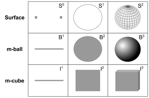
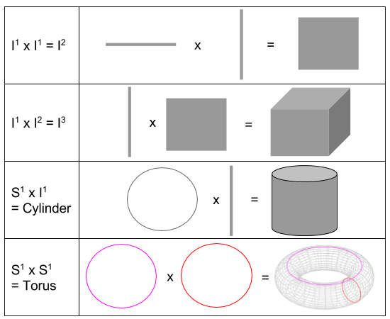
A 1-ball $B^1$ is a line segment
A 2-ball $B^2$ is a disc
$S^1$ is a circle
$S^2$ is a sphere

Note the difference between volumes and their surfaces. Do not confuse e.g., a disc with a circle. The boundary operation $\partial$ makes the volume-surface relationship explicit. For example, we say that $\partial B^2 = S^1$ .

Note that surfaces are one dimension below their corresponding volume. For example, a disc resides on a plane, but a circle can be unrolled to fit within a line.

Importantly, an m-ball and an m-cube are considered equivalent! After all, they can be deformed into one another. This is the reason for the old joke:

A topologist cannot tell the difference between a coffee cup and a donut. Why? Because both objects are equivalent under homeomorphism:

If numbers are the objects of arithmetic, operations like multiplication act on these numbers. Topological operations include product, division, and connected sum. Let us address each in turn.

On Product

The product (x) operation takes two manifolds of dimension m and n, and returns a manifold of dimension m+n. A couple examples to whet your appetite:

Topology- Examples of Product (1)

These formulae only show manifolds of small dimension. But the product operation can just as easily construct e.g. a 39-ball as follows:

$B^{39} = \prod_{i=1}^{39} I^1$

How does product relate to our boundary operator? By the following formula:

$\partial (M x N) = ( \partial M x N) \cup (M x \partial N )$

This equation, deeply analogous to the product rule in calculus, becomes much more clear by inspection of an example:
Topology- Product vs Boundary (1)

On Division

Division ( / ) glues together the boundaries of a single manifold. For example, a torus can be created from the rectangle $I^{2}$ :

torus_by_division

We will use arrows to specify which edges are to be identified. Arrows with the same color and shape must be glued together (in whatever order you see fit).

Topology- Division Simple Examples (2)

Alternatively, we can specify division algebraically. In the following equation, x=0 means “left side of cylinder” and x=1 means right side:

$S^1 x I^1 = Cylinder = \frac{I^2}{(0,y) \sim (1, y) \forall y}$

The Möbius strip is rather famous for being non-orientable: it neither has an inside nor an outside. As M.C. Escher once observed, an ant walking on its surface would have to travel two revolutions before returning to its original orientation.

More manifolds that can be created by division on $I^{2}$ . To construct a Klein bottle by division, you take a cylinder, twist it, and fold it back on itself:

Topology- Klein Bottle Construction (5)

In our illustration, there is a circle boundary denoting the location of self-intersection. Topologically, however, the Klein bottle need not intersect itself. It is only immersion in 3-space that causes this paradox.

Our last example of $I^{2}$ division is the real projective plane $RP^{2}$ . This is even more difficult to visualize in 3-space, but there is a trick: cut $I^{2}$ again. As long as we glue both pieces together along the blue line, we haven’t changed the object.

Topology- Deriving Real Projective Plane First Part (1)

The top portion becomes a Möbius strip; the bottom becomes a disc. We can deform a disc into a sphere with a hole in it. Normally, we would want to fill in this hole with another disc. However, we only have a Möbius strip available.

But Möbius strips are similar to discs, in that its boundary is a single loop. Because we can’t visualize this “Möbius disc” directly, I will represent it with a wheel-like symbol. Let us call this special disc by a new name: the cross cap.

The real projective plane, then, is a cross cap glued into the hole of a sphere. It is like a torus; except instead of a handle, it has an “anomaly” on its surface.

Topology- Deriving Real Projective Plane Second Part

These then, are our five “fundamental examples” of division:

Topology- Division Overview (3)

On Connected Sum

Division involves gluing together parts of a single manifold. Connected sum (#), also called surgery, involves gluing two m-dimensional manifolds together. To accomplish this, take both manifolds, remove an m-ball from each, and identify (glue together) the boundaries of the holes. In other words:

$\frac{ ( M_1 / B_1 ) \cup ( M_2 / B_2 ) }{ \partial ( M_1 / B_1 ) \sim \partial ( M_2 / B_2 )} = M_1 \# M_2$

Let’s now see a couple examples. If we glue tori together, we can increase the number of holes in our manifold. If we attach a torus with a real projective plane, we acquire a manifold with holes and cross-cuts.
Topology- Connected Sum examples (3)

Takeaways

Topology, aka. “rubber sheet geometry”, is the study of malleable objects & spaces.
In topology, manifolds represent objects in n-dimensional space.
Manifolds either represent volumes (e.g., disc) and boundaries (e.g., circles)
Manifolds are considered equivalent if a homeomorphism connects them.
There are three basic topological operations:
- Product (x) is a dimension-raising operation (e.g., square can become a cube).
- Division (/) is a gluing operation, binding together parts of a single manifold.
- Connected sum (#) i.e., surgery describes how to glue two manifolds together.

Related Materials

This post is based on Dr. Tadashi Tokeida’s excellent lecture series, Topology & Geometry. For more details, check it out!

The X-Bar Theory of Phrase Structure

October 2, 2017October 3, 2017kevinbinz 2 Comments

Part Of: Language sequence
Followup To: An Introduction to Generative Syntax
Content Summary: 800 words, 8 min read

Explaining Substitution

Consider the sentence “I bought this big book of poems with the red cover”.

XBar- Flat Noun Phrase (1)

In everyday language, we often replace words and phrases with indexing words like “one”. Call this indexing replacement.The meaning of these words can be obtained from the context.

At first glance, indexing replacement seems to target a branch in the syntax tree. For example:

I bought that big one of poems with the red cover (“one” replaces the noun)
I bought one (“one” replaces the entire noun phrase)

But there are several other substitutions don’t follow from branch replacement:

I bought that big one.
I bought that small one
I bought that big one of poems with the blue cover

Perhaps our notion of noun phrases is too flat. Perhaps we need additional nodes to describe structure within the noun phrase. We will call these intermediate nodes N’, (where N → N’ → N’’ = NP):

towards_noun-bar

This new tree successfully predicts all substitution phenomena, by modeling “one” as replacing various “N-bar” nodes:

xbar_noun_substitution

We can similarly introduce depth to our verb phrases (VPs), by using intermediate V’ (“V-bar”) nodes:

XBar- Verb Substitution (2)

The X-Bar syntax tree provides a simple explanation of the “do so” substitution effects:

I will do so in the office before the party.
I will do so before the party.
I will do so.

A General Theory of Phrases

We can revise our original NP and VP rules to reflect our intermediate N’ and V’ nodes:

Xbar Theory- Towards XBar Rules

What if noun and verb phrases are instantiations of a more general phrase structure? Just as group theory identifies overlap in the axioms of addition and subtraction, X-bar theory explores the similarity between NP and VP rules.

Xbar Theory- XBar Parameterization (1)

There are only four kinds of phrase constituents:

The head carries the central meaning of the phrase. Consider the sentence “The tall student who is wearing the red shirt asked questions of her professor, after the lecture.” The central meaning is retained if we remove all non-head words: “student asked questions”.
The specifier points to the head. For nouns, specifiers include determiners (“the”) and possessives (“her”). For verbs, adverbs occasionally fill this role (“quickly”).
The complement tends to feel intimately related to the head of a phrase (e.g., “of poems” in “a book of poems”).
Adjuncts, on the other hand, tend to feel more optional (e.g., “big” in “big book”).

Xbar Theory- Phrase Structure

Adjuncts vs Complement

Given that adjuncts and complements both often inhabit prepositional phrases, it is perhaps surprising that they should behave differently. The distinction between adjuncts and complements explains why this should be the case. Let us look at four behavioral differences:

Difference #1. Adjuncts can be reordered freely.

Consider our example verb phrase:

Xbar Theory- VBar and NBar Example

This rule means that our two adjuncts can be shuffled, but the complement NP must retain its original position

I will read the letter in the office before the party (Original order: valid)
I will read the letter before the party in the office (Adj reorder: valid)
*I will read in the office before the party the letter (Compl reorder: invalid)

Difference #2. Indexing replacement cannot strand the complement.

For example,

I will do so in the office before the party (Adj is stranded: valid)
*I will do so the letter before the party (Compl is stranded: invalid)

Consider another part of speech we have not yet considered: conjunction words like “and” and “or”.

Difference #3. Conjunction words bind adjuncts together, and complements together. But adjunct-complement bindings are non-grammatical.

Consider our example noun phrase:

Xbar Theory- NBar Example (1)

Three examples to illustrate how conjunction works:

I bought the book of poems and of short stories. (Compl-compl conjunction: valid)
The book with the red cover and the black spine. (Adj-adj conjunction: valid)
*The book of poems and with the red cover. (Compl-adj conjunction: invalid)

What X-Bar Theory Tells Us About Memory

Earlier, I introduced the distinction between episodic and semantic memory:

Semantic: ability to remember facts and concepts (e.g., hands have five fingers)
Episodic: ability to remember events or episodes (e.g., dinner last Tuesday night)

Concepts are learned by extracting commonalities from episodic memories. If you see enough metallic blocks moving around on four cylinders, you’ll eventually consolidate these objects into the CAR concept:

XBar Theory- Semantic vs Episodic Memory

In philosophy, I suspect the concepts of necessity and contingency relate to semantic and episodic memory, respectively.

In linguistics, I suspect complements help locate concepts in semantic memory, whereas adjuncts assist episodic localization. In the sentence “I bought the book of poems with the red cover”, the complement helps us activate the concept POEM-BOOK, whereas the adjunct creates sense-predictions that locate it within our episodic memory.

Takeaways

With flat syntax trees, it is difficult to explain indexing substitution (e.g., “bought a book” → “bought one”)
If we make syntax trees binary, by introducing intermediate X’ (“X-Bar”) nodes, substitution becomes more straightforward.
Noun and verb phrases thus parameterize a more general phrase structure.
Phrases have four kinds of constituents: head, specifier, complement, and adjuncts.
The differences between complements and adjuncts are instructive:
- Only adjuncts can be reordered.
- Indexing replacement cannot strand the complement.
- Conjunction cannot bind across categories
In human cognition, complements and adjuncts may correspond to semantic and episodic memory, respectively.

Logic Design: Harmony in IPL

August 10, 2017August 10, 2017kevinbinz Leave a comment

Followup To: Logic Structure: Connectives in IPL
Part Of: Logic sequence
Content Summary: 300 words, 3 min read

Motivations

Last time, we looked at Intuitionistic Propositional Logic (IPL). In IPL, there are five connectives, and hence five introduction-elimination pairs:

IPL- All Rules (1)

What if you had to design a new logic from scratch? Suppose we were to invent five new connective symbols. Would you start by defining their introduction rule, and use these to infer elimination? Or would you instead define elimination first?

This choice reflects different ways to interpret the semantics of logic:

The verificationist starts with introduction first. For them, the meaning of a connective is in their constructor (introduction rules).
The pragmatist starts with elimination first. For them, the meaning of a proposition is how you use it.

But if introduction and elimination rules agree, then a logical system has harmony.

How do we evaluate harmony in practice? Harmony is defined as two propositions:

Local soundness: if I introduce and then eliminate a connective, do I gain information? If so, the elimination rule is too weak.
Local completeness: if I eliminate then re-introduce connective, do I lose information? If so, the elimination rule is too strong.

Demonstrating Harmony in IPL

We can show that conjunction rules exhibit harmony.

IPL Harmony- Conjunction Connective (1)

Note that we have only shown soundness for left-elimination. But demonstrating soundness for right-elimination is highly analogous.

Implication rules also exhibit harmony.

IPL Harmony- Implication Connective (4)

So does disjunction.

IPL Harmony- Disjunction Connective (5)

It is trivial to demonstrate the harmony of truth and falsity. Thus, we can say that IPL, as a formal system, has harmony.

Takeaways

In this article, we have discussed harmony, which helps us evaluate how useful a given formal system is. This notion may seem straightforward in IPL; however, it will prove useful in designing new logics, such as linear logic.

Another more subtle point to consider is that the soundness demonstration also seems to reflect a logic of simplification. This point will return when we discuss the Curry-Howard-Lambek correspondence, and the deep symmetries between logic and computation.

Until next time.

The Tripartite Mind

July 5, 2017July 5, 2017kevinbinz Leave a comment

Part Of: Neural Architecture sequence
Content Summary: 700 words, 7 min read

Dual-Process Theory

Dual process theory identifies two modes of human cognition: a fast, parallel System 2 and a slow, serial System 1.

Linguistic Implications- Dual Process Theory

This distinction can be expressed phylogenetically:

Tripartite Mind- Dual-Process Theory Phylogeny (2)

But this is incorrect. We know that engine of consciousness is the extended reticular-thalamic activating system (ERTAS), which implements feature integration by phase binding. Mammalian brains contain this device. Also, behavioral evidence indicate that non-human animals possess working memory and fluid intelligence[C13].

Conscious, non-linguistic animals exist. We need a phylogeny that accepts this fact.

The Tripartite Mind

Let’s rename System 1, and divide System 2 into two components.

The Autonomous mind is a subsymbolic neural network.
The Algorithmic Mind constructs perceptual object via the Global Workspace.
The Linguistic Mind applies linguistic processing to conscious contents.

This allows us to conceive of conscious, non-verbal mammals:

Linguistic Musings- Architectural Phylogeny (1)

This lets us refresh our view of property dissociations:

Tripartite Mind- TPM Property Dissociations (1)

Most dual-process theorizing (for example, our theory of moral cognition) maps neatly to the autonomous and linguistic mind, respectively.

But the Tripartite Mind theory cannot bear the weight of all behavioral phenomena. For that, we need the more robust language of two loops. In fact, we can marry these two theories as follows:

Tripartite Mind- Cybernetics Interpretation

This diagram reflects the following facts:

The Autonomous Mind constitutes most of the brain.
The Algorithmic Mind is perceptual, and processes Autonomic representations.
The Linguistic Mind receives Algorithmic (but not Autonomic) information.

Boundaries on the Linguistic Mind

The Linguistic Mind creates cultural knowledge. It is the technology underlying the invention of agriculture, calculus, and computational neuroscience. It is hard to see how such a device could be not only biased, but in some respects completely blind.

But the Linguistic Mind does not have access to raw sensorimotor signals. It only has access to the intricately curated working memory. You cannot communicate mental experiences outside of working memory. You can try, but that would be confabulation (unintentional dishonesty). As [NW77] describe in their seminal paper Telling more than we can know, in practice, human beings are strangers to themselves.

The evidence suggests that working memory does not contain any information about your judgments and decision making. All attempts to describe this aspect of our inner life fail. Introspection on these matters cannot secure direct access to the truth of the matter. Rather, we guess at our own motives, using the exact same machinery we use to interpret the behavior of other people. For more on the Interpretive Sensory Access theory of introspection [C10], I recommend this lecture.

Sociality and the Linguistic Mind

Per the Social Brain Hypothesis [D09], humans are not more intelligent than other primates; we are rather more social. In other words, the Linguistic Mind is a social invention, which facilitates the construction of cultural institutions which allow propriety frames to be synchronized more explicitly.

On the argumentative theory of reasoning, social reasoning is not independent of language. It is the purpose of language.

Argumentative Reason- Module Evolution (2)

While the Linguistic Mind evolved to satisfy social selection pressures, not all primate sociality is linked to this device. Social mechanisms have arrived in stages:

Primary emotions as social behavior network can be traced back to ray-finned fish.
In New World primates, body language evolved as an extension to our autonomic nervous system, as described in the polyvagal theory. [P03]
Certain human-specific social mechanisms evolved within the neuroimmune axis as a defense mechanism to parasites [TF14].

All of these mechanisms can be attributed to the Autonomous Mind. But since the Linguistic Mind is driven by our motivation apparatus (just like everything else in the brain), its behavior is sensitive to the wishes of these “lower” modules. This doesn’t contradict our earlier assumption that its content is divorced from Autonomous data.

References

[C13] Carruthers 2013. Evolution of working memory.
[C10] Carruthers 2010. Introspection: Divided and Partly Eliminated
[TF14] Thornhill, Fincher (2014). The Parasite-Stress Theory of Sociality, the Behavioral Immune System, and Human Social and Cognitive Uniqueness.
[P03] Porges (2003). The Polyvagal Theory: phylogenetic contributions to social behavior
[D09] Dunbar (2009). The social brain hypothesis and its implications for social evolution