Part Of: Game Theory sequence
Content Summary: 1300 words, 13 min read
Prisoner’s Dilemma Review
The classical Prisoner’s Dilemma has following setup:
Two prisoners A and B are interrogated, and separated asked about one another.
- If both prisoners betray the other, each of them serves 2 years in prison
- If A betrays B but B remains silent, A will be set free and B will serve 3 years (and vice versa)
- If both prisoners remain silent, they will only serve 1 year in prison.
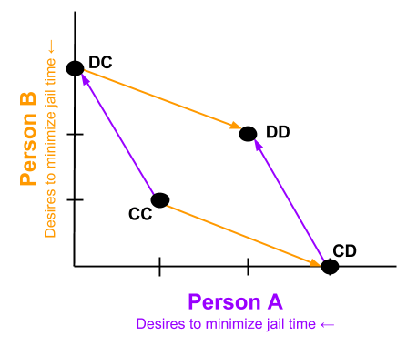
We can express the decision structure graphically:

We can also represent the penalty structure. In what follows, arrows represent preference. CC → DC is true because, given that B cooperates, A would prefer the DC outcome (0 years in prison) more than CC (1 year).
Our takeaways from our exploration of the Prisoner’s Dilemma:
- An outcome is strategic dominance happens when one choice outperforms other choices, irrespective of competitor behavior. Here, DD is strategically dominant.
- Pareto improvement is a way to improving at least one person’s outcome without harming any other player. Here, DD → CC represents such an improvement.
- Pareto optimal outcomes are those outcomes which cannot be Pareto-improved.
The Prisoner’s Dilemma shows us that strategically-dominant outcomes need not be Pareto optimal. Although each arrow points towards the origin for that color, the sum of all arrows points away from the origin.
It packages together the tragedy of the commons, a profound and uncomfortable fact of social living. A person can be incentivized towards an outcome that she, and everybody else, dislikes.
Towards Iterated Prisoner’s Dilemma (IPD)
In the one-off game, mutual defection is the only (economically) rational move. If a person chooses to defect, they will likely receive a bad result.
But consider morwhat happens in a more social setting, where players compete for resources multiple times. An Iterated Prisoner’s Dilemma (IPD) has the following structure:

What strategy is best? Let’s consider two kinds of strategies we might adopt. We can imagine some vindictive prisoners always defecting (AD). Other prisoner’s might be more generous, adopting a Tit-for-Tat (TfT) strategy. This has them initially cooperating, and mirroring their opponent’s previous move.
Let’s imagine that there are 200 “prisoners” playing this game, with each strategy adopted by half of the population. Which strategy should you adopt, in such a scenario?
The games look as follows:
- AD vs AD: { DD, DD, DD, … }. After 10 rounds: A has 20 years, B has 20 years.
- AD vs TfT: { CD, DD, DD, … }. After 10 rounds: A has 18 years, B has 21 years.
- TfT vs TfT: { CC, CC, CC, … }. After 10 rounds: A has 10 years, B has 10 years.
These computations can be generalized to n rounds:

The tit-for-tat (TfT) strategy wins because TfT-TfT games are collaborative, but these players also aren’t effectively exploited by players who Always Defect (AD).
Which Kinds of Strategies Are Best?
There is an very large number of possible IPD strategies. Strategy design might include considerations such as:
- Deterministic vs Mixed. Should we follow logical rules, or employ randomness?
- Impersonal vs Personal. Do we remember the behavior of each opponent? Do we change strategies given what we know of other players?
- Fixed vs Adaptive. Should we use our experiences to change the above on-the-fly?
Given this behavioral diversity, which kinds of strategy are most successful?
To answer this question, in 1980 Robert Axelrod conducted a famous experiment. He invited hundreds of scholars to enter an IPD tournament, submitting their agent’s decision algorithm digitally. In a computer simulation, every agent played every other agent 200 times. The agent with highest cumulative utility was declared the winner.
Many agent strategies employed quite complex, using hundreds of lines of code. The surprising result was that simple strategies, including Tit-for-Tat, often proved to be superior. Axelrod described three properties shared among successful strategies:

We can call such strategies instances of reciprocal altruism.
Moral and Emotional Implications
The theory of evolution has shown us that biological systems are the product of an optimization process known as natural selection. Only genes that improve reproductive success win over evolutionary time.
From this context, it has long seemed unclear how human beings (and other animals) came to express altruistic behavior. W.D Hamilton’s notion of inclusive fitness explains why we behave generously to relatives. As J.B.S Haldane famously joked,
I would willingly die for two brothers or eight cousins.
Game theory explains our behavior towards non-relatives. Specifically,
IPD provides insight into moral cognition. It shows how our selfish genes might, purely for selfish reasons, come to promote behaviors that are (reciprocally) altruistic.
IPD similarly explains certain emotional processes. For example, I have posited elsewhere the existence of social intuition generators like Fairness. We can now explain why natural selection generated such “socially intelligent” mental modules.
Application: Vampire Bats
Instead of jail time, we can modify our outcome structure to be more relevant to biology.
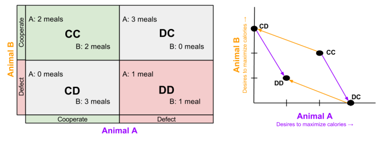
Thus, we can use game theory to interpret animals competing for resources. Consider, for example, behavior of the vampire bats.
Vampire bats feed on the blood of other mammals. Their energy budget is such that they can tolerate 2 days of food deprivation before starving to death.
On a given night, 8% of adult vampire bats will fail to find food on a given night. But when they do find food, it is often more than they need.
Of course, these animals have a genetic incentive to share blood within family. But you can also observe bats sharing their food with strangers.
How can selfish genes reward altruistic behavior? Because vampire bats are playing IPD:
- CC (Reward). I get blood on my unlucky nights. I have to give blood on my lucky nights, which doesn’t cost me too much.
- DC (Temptation). You save my life on my poor night. But I also don’t have to feed you on my good night.
- CD (Sucker): I pay the cost of saving your life on my good night. But on my bad night I still may starve.
- DD (Punishment) I don’t have to feed you on my good nights. But I run a real risk of starving on my poor nights.
Towards Evolutionary Game Theory
To show why altruistic bats are more successful? Yes; we need only invent evolutionary game theory (EGT). Recall how natural selection works:
Individuals with more biological fitness tend to leave more copies of their genes.
EGT simply adds this replicator logic to the Iterated Prisoner’s Dilemma (IPD). Players with higher final scores (most resources) leave more descendants in subsequent populations (image credit):
We saw previously that Tit-For-Tat players outperform those who Always Defect. In EGT, this fact establishes how a gene that promotes altruism successfully invaded the vampire bat gene pool:

Of course, iterated games don’t always have one winner. Consider the following food web (structurally similar to Rock-Paper-Scissors, of course).
Snake beats Fox. Fox beats Hawk. Hawk beats snake.
What if the size of the snake population starts out quite small? In that case, hawks and foxes predominate. Since hawks are prey to foxes, the size of the hawk population decreases. But this means the snakes have fewer natural predators.
The above traces the implications of one possible starting point. However, we can use EGT maths to model the entire dynamical system, as follows (image credit):
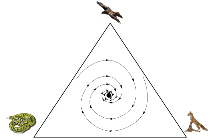
With this image, we can see that any starting point will eventually (after many generations), lead to a (⅓, ⅓, ⅓) divide of snakes, foxes, and hawks. This point is the locus of the “whirlpool”, it is also known as an attractor, or an evolutionarily stable state (ESS).
Takeaways
- The Iterated Prisoner’s Dilemma (IPD) makes game theory more social, where many players compete for resources multiple times.
- While one-off PD games favor selfish behavior, IPD can favor strategies that feature reciprocal altruism, such as Tit-for-Tat.
- More generally, IPD strategies do best if they are nice, retaliating, and forgiving. This in turn explains how certain facets of our social and moral intuitions evolved.
- Evolutionary Game Theory (EGT) extends IPD by adding replicator logic (more successful strategies are preferentially represented in future generations).
- Evolutionary Stable States (ESS) encode dynamical attractors, which populations asymptotically approach.
Until next time.


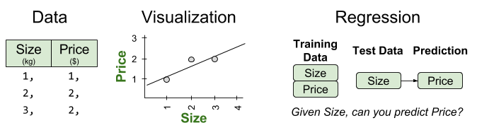
 and a line determined by vector
  , how do we find the point on the line that is closest to
 is at the intersection formed by a line through
  is the error of that approximation.
 and
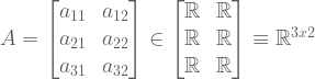
and  . This plane can be described with a matrix, by mapping the basis vectors onto its column space:


 are self-transpositions. We have shown that such matrices are square symmetric, and thereby contain positive, real eigenvalues.
 :
:

 , that accepts a vector


 :
:
 such that the error
  is minimized.
 as small as possible. Since
  can never leave the column space, choose the closest point to
  is the projection of b onto the column space. The error is perpendicular to that subspace. Therefore


 :
:![\bar{x} = \left[ (A^TA)^{-1}A^T \right] b = \begin{bmatrix} 4/3 & 1/3 & -2/3 \\ -1/2 & 0 & 1/2 \\ \end{bmatrix} \begin{bmatrix} 1 \\ 2 \\ 2 \\ \end{bmatrix} = \begin{bmatrix} 2/3 \\ 1/2 \\ \end{bmatrix}](https://s0.wp.com/latex.php?latex=%5Cbar%7Bx%7D+%3D+%5Cleft%5B+%28A%5ETA%29%5E%7B-1%7DA%5ET+%5Cright%5D+b+%3D+%5Cbegin%7Bbmatrix%7D+4%2F3+%26+1%2F3+%26+-2%2F3+%5C%5C+-1%2F2+%26+0+%26+1%2F2+%5C%5C+%5Cend%7Bbmatrix%7D+%5Cbegin%7Bbmatrix%7D+1+%5C%5C+2+%5C%5C+2+%5C%5C+%5Cend%7Bbmatrix%7D+%3D+%5Cbegin%7Bbmatrix%7D+2%2F3+%5C%5C+1%2F2+%5C%5C+%5Cend%7Bbmatrix%7D&bg=ffffff&fg=555555&s=0&c=20201002)


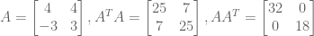
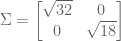
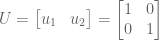
 (with eigenvectors along the columns) and a matrix
  (with eigenvalues along the diagonal).

 as
as  and
and  .
. . Then
  and
and  . So these matrices are square. But they are also symmetric!


 .
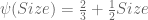
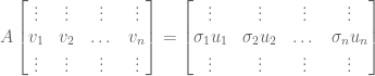
. produces an orthogonal basis in the column space. Orthogonal bases are not particularly hard to find. But most orthogonal bases, once projected to column space, will lose their orthogonality! We desire that particular orthogonal basis
  such that
  , analogous to eigenvalues
  .
. , analogous to diagonal matrix


 ,
,
 . So,
. So,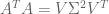


 . The above findings give us two of these ingredients.


 and symmetric
  ).
). . That is, every linear transformation can be conceived as rotation + scaling + rotation.
 degrees.
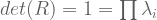
 whose output vectors
  differ by a scaling factor.
 ).
).
 pairs that satisfy the above equality.
 matrix, there are
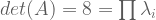
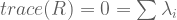
  eigenvalues. These eigenvalues can be difficult to find. However, two facts aid our search:
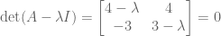
 from both sides:
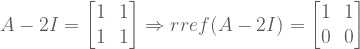
 has an empty nullspace, it will contain zero eigenvectors. So we desire this new matrix to be singular.
 . Matrices are singular iff their determinants equal zero.


 :
:

 :
:


 ?
?
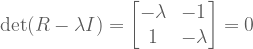
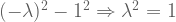
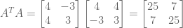
![A = \left[ \begin{smallmatrix} 3 & 1 \\ 1 & 3 \\ \end{smallmatrix} \right]](https://s0.wp.com/latex.php?latex=A+%3D+%5Cleft%5B+%5Cbegin%7Bsmallmatrix%7D+3+%26+1+%5C%5C+1+%26+3+%5C%5C+%5Cend%7Bsmallmatrix%7D+%5Cright%5D&bg=ffffff&fg=555555&s=0&c=20201002) has real eigenvalues, but
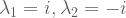
has real eigenvalues, but ![R = \left[ \begin{smallmatrix} 0 & -1 \\ 1 & 0 \\ \end{smallmatrix} \right]](https://s0.wp.com/latex.php?latex=R+%3D+%5Cleft%5B+%5Cbegin%7Bsmallmatrix%7D+0+%26+-1%C2%A0%5C%5C+1+%26+0%C2%A0%5C%5C+%5Cend%7Bsmallmatrix%7D+%5Cright%5D&bg=ffffff&fg=555555&s=0&c=20201002) has less-desirable complex eigenvalues.
has less-desirable complex eigenvalues. as follows:
 . What happens when you multiply the original matrix
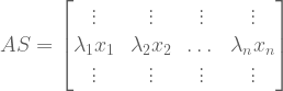


 . Thus, if
 :
:
 :
:
 What is
  ?
?

 .
.


 and
and  . We can then express the Fibonnaci matrix


