Part Of: Algebra sequence
Content Summary: 1300 words, 13 min read.
Linear algebra is the math of vectors and matrices. Let me attempt to explain it as succinctly as possible.
Vector Operations
If n is a positive integer and ℝ is the set of real numbers, then ℝn is the set of all n-tuples of real numbers. A vector v ∈ ℝn is one such n-tuple. For example,

The six vector operations are: addition, subtraction, scaling, cross product, dot product, norm (vector length). For vectors u and v, these are defined as follows:

The dot product and the cross product norm are related to the angle between two vectors. Specifically,


Finally, note the the cross product is not commutative: u x v != v x u.
Matrix Operations
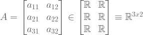
A matrix A ∈ ℝm x n is a rectangular array of real numbers with m rows and n columns. For example,
Important matrix operations are addition, subtraction, product, transpose, and determinant:

Of the above operations, matrix product is especially significant. This operation is only possible when A has the same number of columns as B has rows.
Matrix as Morphism
Importantly, matrices with one row or one column can interpreted as vectors. Matrix multiplication with a vector can be interpreted in two ways. The row picture interprets the output as a dot product, the column picture interprets the output as a linear combination.

Let’s take A to be a 2 by 2 matrix with row-vectors (2, -1) and (-1,2), and let b = (0,3). When we solve for x, we find there are two ways to do so:

In the above example, we set b = (0,3). But this linear combination could generate any vector b. In general, linear combinations can generate the entirety of a space (in this case, a two-dimensional plane).
In both views, we say A transform x → b. If vectors are groups of data, matrices are functions that operate on vectors. Specifically, multiplication by a matrix A ∈ ℝm x n we will call a linear transformation, that converts an n-tuple into a m-tuple TA : ℝn → ℝm.
The symmetry between functions and linear transformations runs deep. When we explore category theory, we will discover the structure underpinning this relationship. But in the meantime, consider the following equivalences:

Especially important to matrix functions is the notion of inverse matrix. Just as f-1(x) = ln(x) undoes the effects of f(x) = ex, inverse matrix A-1 undoes the effects of A. The cumulative effect of applying A-1 after A is the identity matrix A-1A = 1. The identity matrix is analogous to multiplying by one, or adding zero: it is algebraically inert.
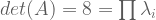
Only square matrices can be invertible, because reversal is commutative AA-1 = A-1A = 1. But not all square matrices have inverses. The determinant of a matrix checks for invertibility. Det(A) != 0 iff A is invertible.
Matrix inversion is vitally important to solving systems of linear equations.
- AX = B → multiply both sides by A-1 on the right → X = A-1B
- XA = B → multiply both sides by A-1 on the right → X = BA-1
- ABXC = E → put C-1 on the right and B-1A-1 on the left → X = B-1A-1EC-1
Elimination As Inverse Solver
To solve Ax = b, we must find inverse matrix A-1. This can be done via Gauss-Jordan Elimination. This method affords three row operations:
- Linear Combination: Ri += kRj
- Scaling: Ri *= k
- Row Swap: Ri ⇆ Rj
After creating a matrix of the form Ax = b, we can solve for x by creating an augmented matrix of the form [ A | b ], and converting the left-hand side into the identity matrix:

To solve for x algebraically, Ax = b → A-1Ax = A-1b → 𝟙x = A-1b. So Gauss-Jordan facilitates the discovery of inverse matrix A-1. We can show this computation explicitly, by setting an augmented matrix of form [ A | 1 ]

![]() Row operations are functions that act on vectors. So are matrices. Thus, it isn’t very surprising that our three row operations each correspond to an elementary matrix. The elementary matrix is similar to the identity matrix; in the below picture, only the shaded region diverges.
Row operations are functions that act on vectors. So are matrices. Thus, it isn’t very surprising that our three row operations each correspond to an elementary matrix. The elementary matrix is similar to the identity matrix; in the below picture, only the shaded region diverges.

We now see that the row operations of Gauss Jordan elimination are a kind of factoring: we are finding the elementary matrices underlying A-1:
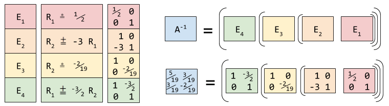
Thus E4E3E2E1 = A-1 and Ax = b → (E4E3E2E1)Ax = (E4E3E2E1)b → x = A-1b
Fundamental Vector Spaces
A vector space consists of a set of vectors and all linear combinations of these vectors. The set of all linear combinations is called the span. For example, the vector space S = span{ v1, v2 } consists of all vectors of the form v = ɑv1 + βv2, where ɑ and β are real numbers.
Vector spaces can be characterized by a basis: the original set of vectors whose linear combination creates the vector space. The vectors of any basis must be linearly independent, or orthogonal. You can check whether two vectors or orthogonal by confirming their dot product u · v = 0. The dimension of a vector space is the cardinality of the basis (number of orthogonal vectors).
Recall that matrices are functions that project vectors from ℝn to ℝm. This corresponds to projecting from row space to column space, as follows:

We will unpack the full implications of this graphic another time. For now, it suffices to understand that discovering the bases of these subspaces is a useful exercise.
For example, if we show that a matrix has an non-empty kernel, this in itself is proof of non-invertibility. Why? Because if TA sends a vector to the zero vector, there is no TA-1 that can undo this operation.
We can say more. For an n x n matrix A, the following statements are equivalent:
- A is invertible
- The determinant of A is nonzero.
- The RREF of A is the n x n identity matrix
- The rank of the matrix is n
- The row space of A is ℝn
- The column space of A is ℝn
- A doesn’t have a null space (only the zero vector N(A) = {0} )
Elimination as Basis Identifier
We have seen elimination discover (and factorize) the matrix inverse. But what happens when an inverse does not exist? Well, elimination has a natural, unique stopping point:

Matrices in reduced row echelon form (RREF) have the following properties:
- Rows with all zeroes are moved to the bottom.
- The first nonzero number from the left (pivot) is to the right of the pivot above it.
- Every pivot equals 1 and is the only nonzero entry in its column
Gauss-Jordan Elimination can replace every matrix with an equivalent one in rref form. Note that we have seen several examples of elimination creates the identity matrix 1 when A is invertible. This is only possible because 1 fits the rref criteria.
Once a matrix is in rref form, it becomes trivial to discover the basis for its three fundamental spaces:
- R(A) basis: all row vectors that are non-zero
- C(A) basis: all column vectors that contain pivot.
- N(A) basis: the solution to Ax = 0

We see that rank(A) + nullity(A) = 3 + 1 = 4, which indeed is the number of columns. Also, the column space of A equals the row space of AT. This is not an accident, since transpose simply swaps rows with columns.
Takeaways
- Vectors are groups of numbers; matrices are functions that act on vectors.
- We can solve linear equations by conducting Gauss-Jordan elimination.
- Gauss-Jordan elimination-based solution rely on searching for inverse matrix A-1
- The domain of matrices is its row vectors, its codomain is its column vectors.
- Even if a matrix is not invertible, elimination can find its most reduced form (RREF).
- RREF matrices can be used to derive fundamental subspaces.
Until next time.
Related Works

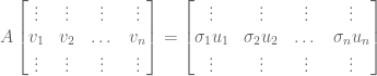
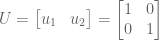
 (with eigenvectors along the columns) and a matrix
  (with eigenvalues along the diagonal).

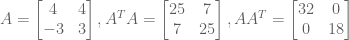
 as
as  and
and  .
. . Then
  and
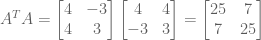
and  . So these matrices are square. But they are also symmetric!


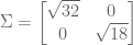
 .
. produces an orthogonal basis in the column space. Orthogonal bases are not particularly hard to find. But most orthogonal bases, once projected to column space, will lose their orthogonality! We desire that particular orthogonal basis
  such that
  , analogous to eigenvalues
  .
. , analogous to diagonal matrix


 ,
,
 . So,
. So,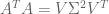


 . The above findings give us two of these ingredients.


 and symmetric
  ).
). . That is, every linear transformation can be conceived as rotation + scaling + rotation.
 degrees.
 whose output vectors
  differ by a scaling factor.
 ).
).
 pairs that satisfy the above equality.
 matrix, there are
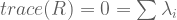
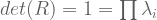
  eigenvalues. These eigenvalues can be difficult to find. However, two facts aid our search:
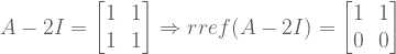
 from both sides:
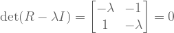
 has an empty nullspace, it will contain zero eigenvectors. So we desire this new matrix to be singular.
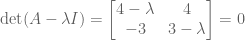
 . Matrices are singular iff their determinants equal zero.


 :
:

 :
:


 ?
?
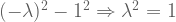
![A = \left[ \begin{smallmatrix} 3 & 1 \\ 1 & 3 \\ \end{smallmatrix} \right]](https://s0.wp.com/latex.php?latex=A+%3D+%5Cleft%5B+%5Cbegin%7Bsmallmatrix%7D+3+%26+1+%5C%5C+1+%26+3+%5C%5C+%5Cend%7Bsmallmatrix%7D+%5Cright%5D&bg=ffffff&fg=555555&s=0&c=20201002) has real eigenvalues, but
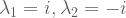
has real eigenvalues, but ![R = \left[ \begin{smallmatrix} 0 & -1 \\ 1 & 0 \\ \end{smallmatrix} \right]](https://s0.wp.com/latex.php?latex=R+%3D+%5Cleft%5B+%5Cbegin%7Bsmallmatrix%7D+0+%26+-1%C2%A0%5C%5C+1+%26+0%C2%A0%5C%5C+%5Cend%7Bsmallmatrix%7D+%5Cright%5D&bg=ffffff&fg=555555&s=0&c=20201002) has less-desirable complex eigenvalues.
has less-desirable complex eigenvalues. as follows:
 . What happens when you multiply the original matrix
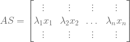


 . Thus, if
 :
:
 :
:
 What is
  ?
?

 .
.


 and
and  . We can then express the Fibonnaci matrix


 is always smaller than
  , because we know all variables are positive. So we have an upper bound OPT ≤ 6. We can sharpen this upper bound, by comparing the objective function to other linear combinations of the constraints.
 . What values of these variables give us the smallest upper bound? Importantly, this is itself an objective function:
 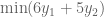 .
. and
and  are constrained: they must produce an equation that exceeds


 and
and 


 . But this is not always the case. In fact, the optimal dual value can be smaller .


![P[a \leq X \leq b] = \int f_X(x) dx](https://s0.wp.com/latex.php?latex=P%5Ba+%5Cleq+X+%5Cleq+b%5D+%3D+%5Cint+f_X%28x%29+dx&bg=ffffff&fg=555555&s=1&c=20201002)


