
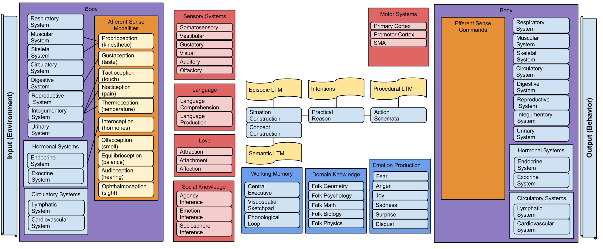
Visceral Neuroanatomy
Stress Sequence
Specific Emotions
Old Material
Visceral Neuroanatomy
Stress Sequence
Specific Emotions
Old Material
Main Sequence
Central Organizing Principles
Main Sequence
Version Iterations
Core Sequence
Bayesian Statistics
Part Of: Optimization sequence
Content Summary: 800 words, 8 min read.
Today, I introduce the concept of duality. Buckle your seat belts! 🙂
Max Flow algorithm
The problem of flow was originally studied in the context of the USSR railway system in the 1930s. The Russian mathematician A.N. Tolstoy published his Methods of finding the minimal total kilometrage in cargo-transportation planning in space, where he formalized the problem as follows.
We interpret transportation graphically. Vertices are interpreted as cities, and edges are railroads connecting two cities. The capacity of each edge was the amount of goods that particular railroad could transport in a given day. The bottleneck is solely the capacities, and not production and consumption. We assume no available storage at the intermediate cities.
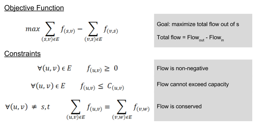
The flow allocation problem defines source and termination vertices, s and t. We desire to maximize volume of goods transported s → t. To do this, we label each edge with the amount of goods we intend to ship on that railroad. This quantity, which we will call flow, must respect the following properties:
Here are two possible solutions to flow allocation:
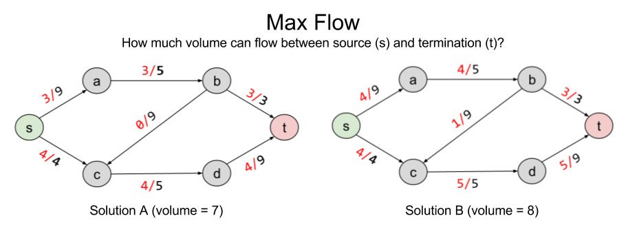
Solution B improves on A by pushing volume onto the b → c railway. But are there better solutions?
To answer rigorously, we formalize max flow as a linear optimization problem:
The solution to LP tells us that no, eight is the maximum possible flow.
Min Cut algorithm
Consider another, seemingly unrelated, problem we might wish to solve: separability. Let X ⊂ E represent the number of edges you need to remove to eliminate a connection s → t. Here are two such solutions:
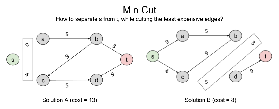
Can we do better than B? The answer is no: { (b,t), (c,d) } is the minimum cut possible in the current graph. In linear programming terms, it is the Best Feasible Solution (BFS)
Note that the BFS of minimum cut and the BFS of max flow arrive at the same value. 8 = 8. This is not a coincidence. In fact, these problems are intimately related to one another. What the min cut algorithm is searching for is the bottleneck: the smallest section of the “pipe” from s → t. For complex graphs like this, it is not trivial to derive this answer visually; but the separability algorithm does the work for us.
The deep symmetry between max flow and min cut demonstrates an important mathematical fact. All algorithms come in pairs. For this example, we will call max flow and min cut the primal and dual problems, respectively. We will explore the ramifications for this another time. For now, let’s approach duality from an algebraic perspective.
Finding LP Upper Bound
Consider a linear program with the following objective function:
And these constraints
This program wants to find the largest solution possible given constraints. Can we provide an upper bound on the solution?
Yes. We can immediately say that the solution is no greater than 6. Why? The objective function, 

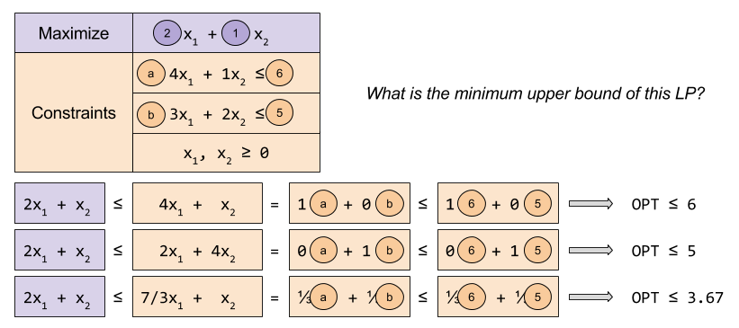
Different weights to our linear combinations produce different upper bounds:
Let us call these two weights 
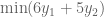
But 


This gives us our two constraints. Thus, by looking for the lowest upper bound on our primal LP, we have derived our dual LP:
Note the extraordinary symmetry between primal and dual LPs. The purple & orange values are mirror images of one another. Further, the constraint coefficient matrix has transposed (the 3 has swapped along the diagonal). This symmetry is reflected in the above linear algebra formulae.
A Theory of Duality
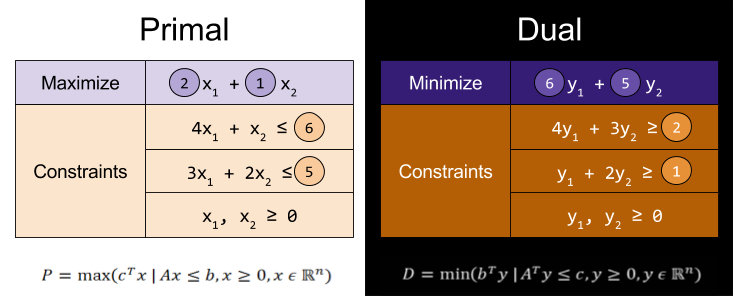
Recall that linear programs have three possible outcomes: infeasible (no solution exists), unbounded (solution exists at +/-∞) or feasible/optimal. Since constraints are nothing more than geometric half-spaces, these possible outcomes reflect three kinds of polyhedra:
The outcome of primal and dual programs are predictably correlated. Of the nine potential pairings, only four can actually occur:
Finally, in the above examples, we saw that the optimal dual value 
We can distinguish between two kinds of duality:


Takeaways
Today, we have illustrated a deep mathematical fact: all problems come in pairs. Next time, we will explore the profound ramifications of this duality principle.
Related Resources: CMU Lecture 5: LP Duality
Part Of: Information Theory sequence
Followup To: An Introduction To Communication
Content Summary: 900 words, 9 min read
Motivations
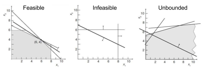
Information theory was first conceived as a theory of communication. An employee of Bell Labs, Shannon was interested in the problem of noise. Physical imperfections on your data cable, for example, can distort your signal.
How to protect against noise? One answer is to purchase better equipment.
But there is another, less expensive answer. Errors can be reduced by introducing redundancy into their signals. But redundancy has a price: it also slows the rate of communication.
Shannon strove to understand this error vs rate trade-off quantitatively. Is error-free communication possible? And if so, how many extra bits would that require?
Before we can appreciate Shannon’s solution, it helps to understand the basics of error correcting codes (ECC). We turn first to a simple ECC: replication codes.
Replication Codes
Error correcting codes have two phases: encoding (where redundancy is injected) and decoding (where redundancy is used to correct errors)
Consider repetition code R3, with the following encoding scheme:
0 → 000
1 → 111
Decoding occurs via majority rule. If most bits are zero the original bit is a 0, and vice versa. Explicitly:
000, 001, 010, 100 → 0
111, 110, 101, 011 → 1
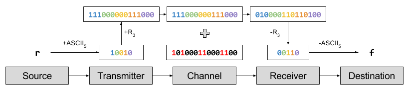
Suppose I want to communicate the word “red” to you. To do this, I encode each letter into ASCII and send those bits over the Internet, to be consumed by your Internet browser. Using our simplified ASCII: ‘r’ → 10010. To protect from noise, we repeat each bit three times: 10010 → 111000000111000.
Let us imagine that 6 bits are flipped: 101000110001100. The last error caused the code 000 → 100, which the decoding algorithm successfully ignores. But the first two noise events caused 111 → 010, which causes a decoding error. These decoding errors in turn change the ASCII interpretation. This pattern of noise will cause you to receive the word “fed”, even though I typed “red”.
Analysis of Repetition Codes
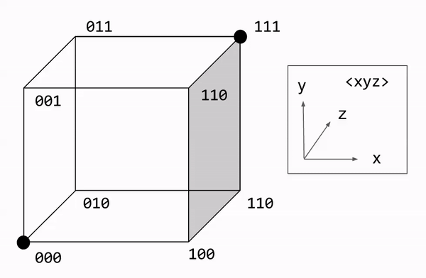
Let us formalize the majority rule algorithm. Decoding involves counting the number of bit flips required to restore the original message. We express this number as the Hamming distance. This can be visualized graphically, with each bit corresponding to a dimension. On this approach, majority rule becomes a nearest neighbor search.
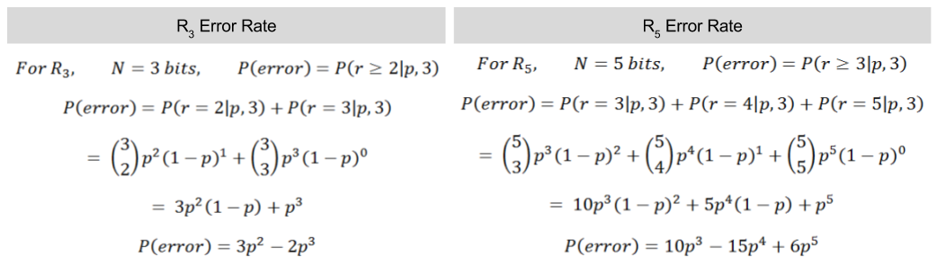
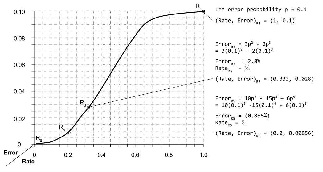
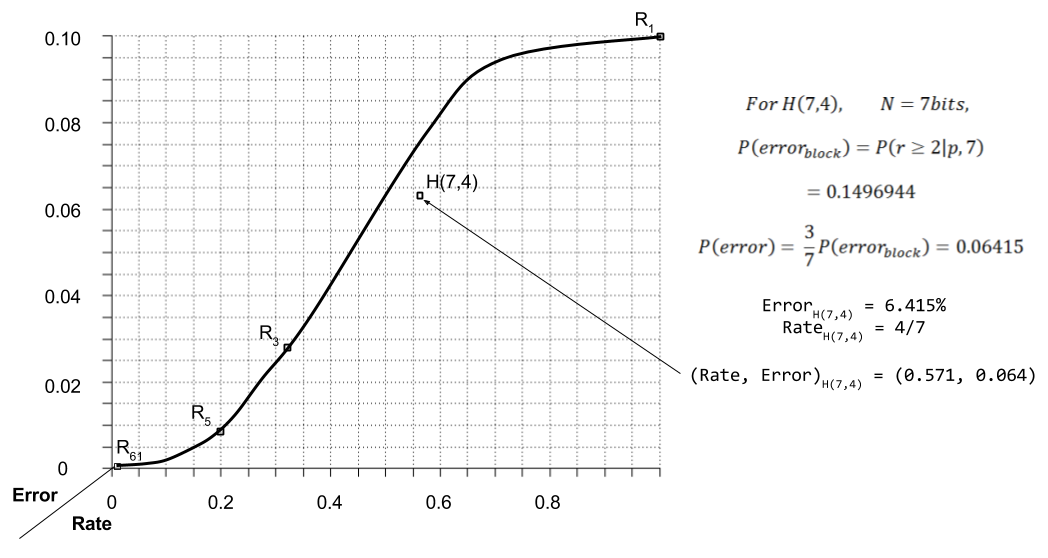
What is the performance of R3? Let us call noise probability p, the chance of any one bit flip. We can model the total number of errors with the binomial distribution:
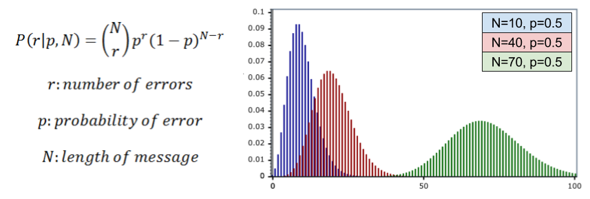
In R3, a decoding error requires two bit flips within a 3-bit block. Thus, P(error) = P(r >= 2|p, 3). We can then compute the frequency of decoding errors.
For p = 10% error rate, we can graph R3 vs R5 performance:
Hamming Codes
In error correcting codes, we distinguish redundant bits versus message bits. Replication codes have a very straightforward mapping between these populations. However, we might envision schemes where each redundant bit safeguards multiple message bits.
Consider the Hamming code, invented in 1950. Richard Hamming shared an office with Claude Shannon for several years. He is also the father of Hamming distance metric, discussed above.
Hamming codes split messages into blocks, and add redundant bits that map to the entire block. We will be examining the H(7,4) code. This code takes 4-bit blocks, and adds three redundant bits at the end. Each redundant bit then “maps to” three of the message bits:
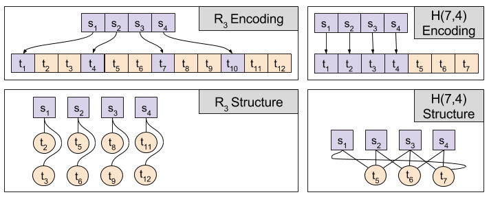
We now define the encoding and decoding algorithms for Hamming Codes. Let message bits s ∈ S be organized into blocks. Let each redundant bit t ∈ T map to a particular subset of the block. For example, s(t7) → { s3, s4, s1 }.
For H(7,4) code, each redundant bit maps to a set of three message bits. If there are an odd number of 1s in this set, the redundant bit is set to 1. Otherwise, it is set to zero. Binary addition (eg., 1+1=0) allows us to express this algebraically:
ti = ∑ s(ti)
A Venn diagram helps to visualize this encoding: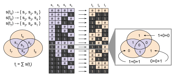
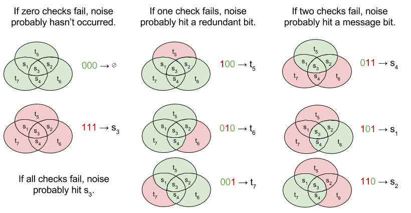
H(7,4) decoding is complicated by the fact that both message bits and redundant bits can be corrupted by noise. We begin by identifying whether there are any inequalities between ti versus ∑ s(ti). If there is, that means *something* has gone wrong.
For H(7,4), there are three redundant bits in every block; there are thus eight different syndromes (error signatures). The decoding algorithm must respond to each possible syndrome, as follows:
The error rate for H(7,4) is calculated as follows.
Application To Information Theory
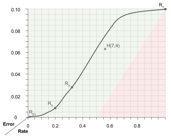
This example demonstrates that Hamming codes can outperform replication codes. By making the structure of the redundant bits more complex, it is possible to reduce noise while saving space.
Can error-correcting codes be improved infinitely? Or are there limits to code performance, besides human imagination?
Shannon proved that there are limits to error-correcting codes. Specifically, he divides the error-rate space into attainable and unattainable regions:
Another important result of information theory is the design of decoding algorithms. Decoding H(7,4) is perhaps the most complex algorithm presented above. For more sophisticated ECCs, these decoding tasks become even more difficult.
Information theory provides a principled way to automate the discovery of optimal decoding algorithms. By applying the principle of maximum entropy, we can radically simplify the process of designing error-correcting codes.
We will explore these ideas in more detail next time. Until then!
Part Of: Neuroeconomics sequence
Content Summary: 8min reading time, 800 words
Reward Prediction Error
An efficient way to learn about the world and its effect on the organism is by utilizing a reward prediction error (RPE) signal, defined as:
The RPE is derived from the Bellman equation, and captures changes in valuation across time. It is thus an error term, a measure of surprise; these are the lifeblood of learning processes.
Phasic dopamine bursts are the vehicle for the RPE signal.
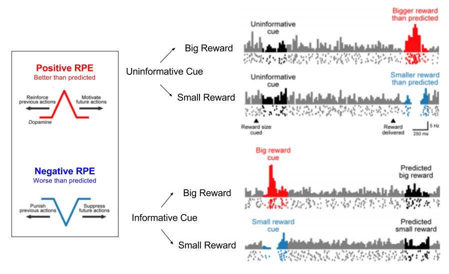
During behavioral conditioning, an animal learns that a behavior is predictive of reward. In such a learning environment, we can see the RPE “travelling forward” in time, until it aligns with cue onset.
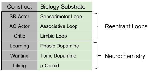
Actors and Critics
The RPE signal is used to update the following structures:
These functions can be computed separately. We call actor the process that updates the policy, and critic the process that updates the value function.
In fact, actors come in different flavors:
Model-based approaches to reinforcement learning are outcome-directed, and encode Action-Outcome (AO) Learning. In contrast, model-free approaches correspond to psychological notions of habit, and behaviorist notions of Stimulus-Response (SR) Learning.
If an animal is using an AO Actor, when they see a reward being moved, they immediately update their model and move towards the new location. In contrast, an SR Actor will learn much more slowly, and require several failed attempts at the old solution before updating its reward topography. Animals show evidence for both behaviors.
The above structures are directly implemented in the three loops of the basal ganglia. Specifically, the AO Actor, SR Actor, and Critic are identified as the Associative, Sensorimotor, and Limbic loops, respectively.
We might define habituation as decisions once handled the AO Actor moved to the SR actor. Correspondingly, when brains learn a habit, we see neural activity transition, from the Associative to the Sensorimotor loop.
Wanting and Liking
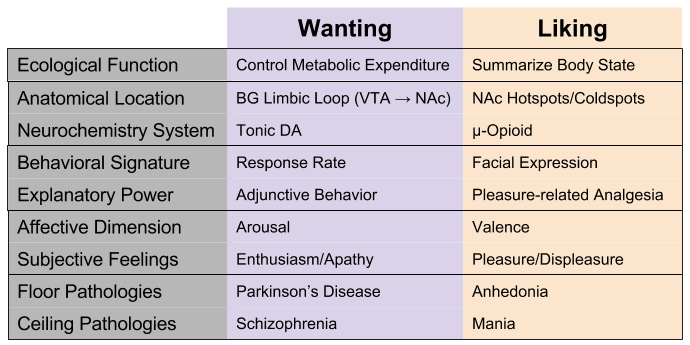
But there is more to reward than learning. Reward also relates to two other processes: wanting (motivation) vs liking (hedonics).
Wanting can be measured by response rate. Strong evidence identifies response vigor (incentive salience) with tonic dopamine levels within the basal ganglia Limbic Loop (VTA to NAc). High tonic dopamine is associated with subjective feelings of enthusiasm, whereas low levels induce apathy. Pathologically high levels of tonic DA are expressed in schizophrenic delirium, pathologically low levels in Parkinson’s disease (disinterest in movement, thought, etc).
Wanting is the substrate of arousal, or motivation. Its purpose is to controls metabolic expenditure. We can see evidence for this in adjunctive behaviors: a severely hungry rat is highly aroused: if food is out of reach, it will still engage in ritualistic behaviors, such as pacing, gnawing wood, or run excessively. Since they are highly aroused, and consummatory behavior is impossible, this “energy” spills out in unrelated behaviors.
Pleasure and displeasure reactions can be measured by unique facial expressions. Strong evidence identifies liking systems with opioid neurochemistry, as expressed by hot/coldspots in the nucleus accumbens (NAc). This system produces subjective feelings of pleasure and displeasure. Pathologically high levels of opioids (morphine-like substances) results in mania; the converse is comorbid with anhedonia.
We can say that opioids collates information about hunger, thirst, pain, etc into a summary statistic of body state.
Takeaways
Reinforcement learning predicts the existence of three learning structures: an SR Actor which behaves habitually, and AO Actor which behaves in accordance to a model, and a Critic that performs outcome valuation. These three structures are implemented as the three reentrant loops in the basal ganglia.
Besides the directive effects of learning, reward also stimulates wanting (i.e., arousal) and liking (i.e., valence). These functions are implemented as three distinct neurochemical mechanisms.
Related Works
I highly recommend the following papers, which motivate our discussion of reentrant loops and neurochemistry, respectively.
You might also explore the following, for a contrary opinion:
So, over the summer I took it upon myself to teach a class on Bayesian Data Analysis, based on the following text,

This was a class put together for several coworkers, including members of our research team at Tableau. Here is a blurb summarizing course content:
Tableau provides various statistical methods, including primitives like Trend Lines (Regression). Our native solutions tend to use rely on Null Hypothesis Significance Testing, which are related to p-values, and a frequentist interpretation of probability. However, Bayesian Statistics is an alternative approach, that has been slowly been gaining traction in several fields.
This class introduced the technical details of Bayesian statistics. It ran July 19 – Sept 27, 2016 and used Doing Bayesian Data Analysis, Second Edition.
- Weeks 1-3 will motivates the Bayesian approach to statistics.
- Weeks 4-7 will give you tools to implement Bayes in R.
- Weeks 8-10 will show how to use Bayesian alternatives to t-tests, regression, and ANOVA.
It was a great experience!
| Week | Chapter | Date | Slides Available |
| 1 | Ch2: Intro to Bayesian Reasoning | July 19 | Yes |
| 2 | Ch4: Intro to Probability Theory | July 26 | Yes |
| 3 | Ch5: Intro to Bayes Theorem | Aug 2 | No |
| 4 | Ch7: Markov Chain Monte Carlo (MCMC) | Aug 9 | Yes |
| 5 | Ch9: Hierarchical Models | Aug 23 | Yes |
| 6 | Ch11: Bayesianism vs Frequentism | Aug 30 | No |
| 7 | Ch16: Bayesian t-test | Sept 6 | No |
| 8 | Ch17: Bayesian linear regression | Sept 20 | Yes |
| 9 | Ch19: Bayesian 1-way ANOVA | Sept 27 | Yes |
Your mileage may vary with the slides, of course. They work best in presentation mode – otherwise some of the transitions are a bit jumpy. I constructed these by myself, with lots of help from our textbook.
Part Of: Demystifying Physics sequence
Followup To: Deep Time
Content Summary: 1100 words, 11 min reading time.
Why does the Earth orbit a slow-burning hydrogen bomb? And why is the night sky illuminated with trillions of such explosions?
Let’s find out.
Preliminaries
Stars emit light. The most important characteristics of light are brightness and color. A Hertzsprung-Russell (HR) Diagram puts brightness on the x-axis, and color on the y-axis. In this way, a star can be represented by a single point.
What happens if you plot the location of all visible stars onto the same HR diagram? The result is rather striking:
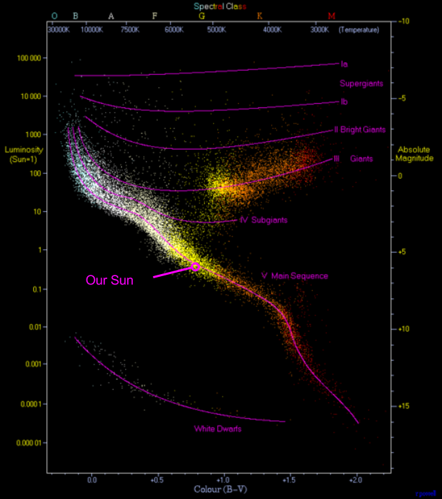
Most stars seem to fit inside a continuous swathe known as the Main Sequence. Why?
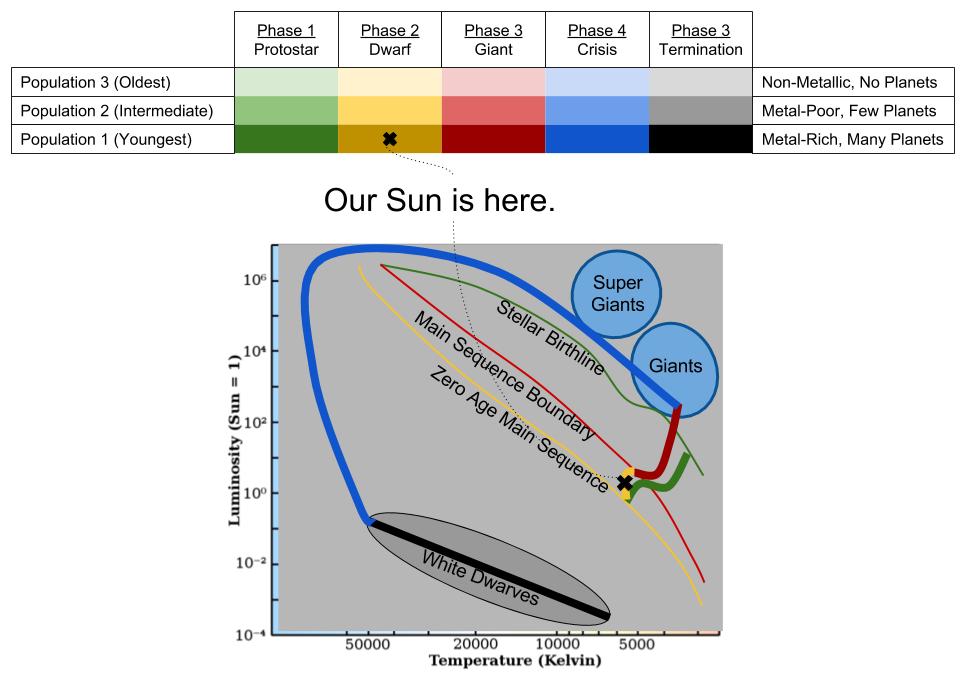
As we will see, there are five stages in the stellar lifecycle:
Stars spent 90% of their lives as dwarves. The radiation of dwarves vary continuously based on solar mass. This explains the Main Sequence.
As we will see, the five life-stages of the stars differ based on how big they are:

The Dynamics of Stars
Stars are born when hydrogen clouds begin to collapse in on themselves.
If gravity was the only force in play, all stars would quickly become black holes. But compressed gases develop high outward pressure. So there are a tension:

Phase 1: Protostars
Star formation begins when a molecular cloud begins to collapse into a dense core. As this core accretes mass, gravity’s pull intensifies. Soon, the site of collapse becomes a protostar.
Protostars are not yet hot enough to induce fusion. But the compression of gravity still makes these objects extremely hot. Once their radiation blows away surrounding clouds, the appear on what is called the stellar birthline of the HR diagram.
As protostars mature, they become more hot and dense. On the HR diagram, their signatures will move from the stellar birthline towards the main sequence.

HR movement is not movement in space. “Travel” away from the stellar birthline means that protostars are growing hotter (left) but less bright (down).
Phase 2: Dwarves (Main Sequence)
The interior of the Sun is not homogenous. The closer to the center, the more extreme the climate. If the protostar is large enough, the core of the star will become so intense, that it will trigger nuclear fusion, releasing enormous amounts of energy. If space was not a vacuum, and the sound of the Sun could travel to Earth, its volume would equal that of a motorcycle.
Nuclear fusion { hydrogen → helium } depletes hydrogen, and creates helium. The helium core of the star expands, as hydrogen is depleted.
Over 90% of a star’s lifetime is spent in this dwarf phase.

Stars are the crucible of matter. What does this mean?
The Primordial Era produced only hydrogen clouds, intermixed with helium. How is it possible for our bodies to be 65% oxygen? Hydrogen does not spontaneously become oxygen, after all.
With few exceptions, all naturally occurring substances were forged in the heart of stars. Nucleosynthesis describes how the raw material of the Big Bang was forged into the chemically diverse world of modernity. In the dwarf phase, we only see the construction of helium. We will soon see nuclear fusion carried much further.

We are literally made of starstuff.
Phase 3: Giants
Eventually, stars run out of hydrogen fuel. At this point, helium atoms are so hot that they start to fuse: { helium → carbon }. This new kind of fusion changes the thermal output of the star, which leaves the main sequence.
Helium-burning stars expand dramatically. For this reason, we call main-sequence stars dwarves, and post main-sequence stars giants.
Again we see a difference along solar mass:

The interior of red supergiants, therefore, is shaped a bit like an onion, with each deeper layer “raising” the atomic number of its exterior. But why does this chain stop at iron?
Iron has the lowest mass per quark: fusing iron consumes energy, instead of creating it.

Small Stars: Fuel Crisis & Termination
Red giants eventually radiate away most of their mass. 😦 Thus, gravity slowly loses its hold on the star, and the outer shells are propelled outward by thermal pressure. This ejection of inert hydrogen is known as a planetary nebula.
The abandoned cores of a shell comprise white dwarves. Since these objects have no source of fuel, they slowly cool, resulting in down-right movement on a HR diagram:

Large Stars: Fuel Crisis & Termination
In contrast to smaller stars, supergiants die in fantastic ways. Their iron core is unstable, and will eventually explode in a supernova. Supernovae are no trifling matter. Their outputs are often brighter than their host galaxies (trillions of stars). If a nearby star in the Milky Way were to go supernova, it would obliterate the human race.

If the core survives the explosion, it becomes a neutron star. Neutron stars are rather dense. One teaspoon of its material would weigh more than ten Pyramids of Giza. Neutron stars are highly magnetic, and rotate quite swiftly: this is the root cause of quasars.
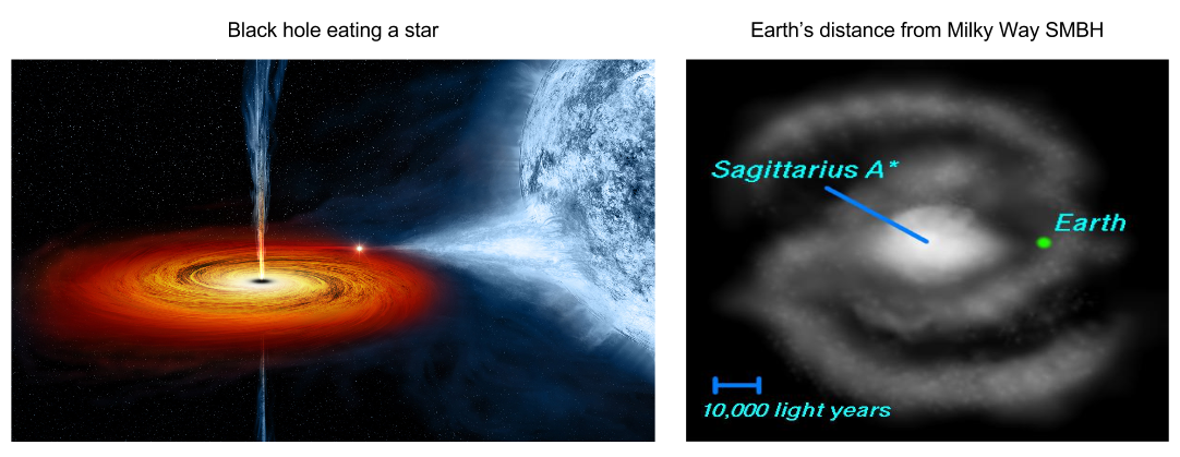
But sometimes the core will be even more dense. In this scenario, it will fully collapse into itself; ripping the fabric of spacetime to become a black hole. Black holes are a bit like predators; they “hunt” and “eat” other stars. At their center, most galaxies possess a supermassive black hole (SMBH). Our galaxy’s SMBH (Sagittarius A*) is fortunately 26,000 light-years away from Earth.
The Story of Our Sun
As we have seen, the universe is 13.8 billion years old, and stars began to form 13.4 billion years ago. We can categorize stars by birthday into three stellar populations.
The earliest stars were chemically simple because the universe contained nothing but hydrogen and helium. But as nucleosynthesis progressed, the universe began to accumulate more complex atoms. The second generation of stars had small amounts of metal. The last generation had substantial metal content.
Did you know that planets outnumber stars? There are about 200 billion stars in the Milky Way, and about 220 billion planets.
Planets are recent inventions. They are created only if a nebula sufficiently high metallic content. In that case, a protoplanetary disc will orbit the protostar, which will ultimately condense into extrastellar satellites.
As a recently-created star, born only 4.6 billion years ago, the Sun’s birthing nebula was sufficiently metallic to create such a disc. This disc eventually consolidated into our eight planets. The Sun is now in its second phase of life, a yellow dwarf. 5.5 billion years from now, it will – like so many of its brothers and sisters – start burning helium as a red giant.
Takeaways
Until next time.
Part Of: Anthropogeny sequence
Content Summary: 900 words, 9min read
Introduction
Primates are relatively young branch of the mammalian clade. Their anatomical characteristics are as follows:

There are three kinds of primate: prosimians (e.g., lemurs), monkeys (e.g., macaques), and apes (e.g., humans).
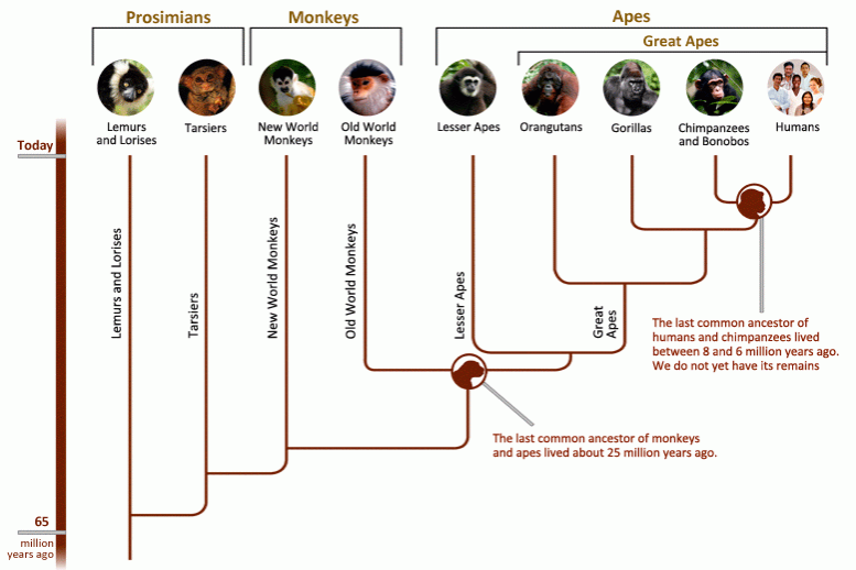
Primates are known for their large brains and a social lifestyle. Today, we will explore the dynamics of primate societies (defined as frequently interacting members of the same species).
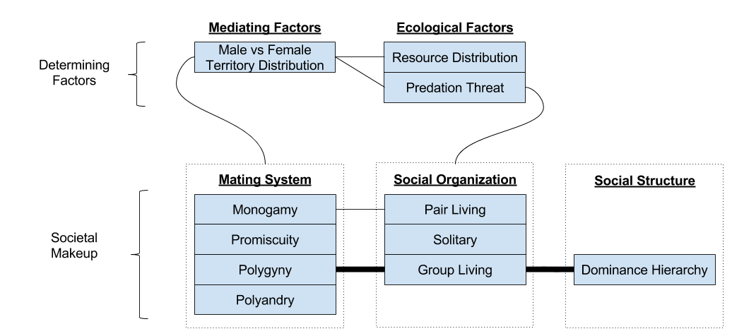
There are three components of any society: the mating system (including sexual dynamics), the social organization (spatiotemporal organization of interaction), and the social structure (relational dynamics & social roles).
Sexual Dynamics
Because DNA is creepy, it programs bodies to make more copies of itself. Men and women are programmed with equally strong imperatives for gene replication (reproductive success). But female pregnancy powerfully breaks the symmetry:
It is because of pregnancy that males court females, and females choose males.
For females, paternal care is of tantamount importance: finding a mate willing to share the burden of raising a child. For males, fecundity is key.
We can see echoes of this asymmetry today. In all human cultures observed,
These gender differences arise as a response to the biological mechanism of pregnancy. These are contingent facts, nothing more. Species with male gestation, such as the seahorse, witness the reversal of such “gender roles”.
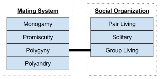
Four Mating Systems
From a logical perspective, there are exactly four possible mating systems.

Which mating system is biologically preferable? That depends on your gender:
Most primates are polygynous. Why?
The answer is geographic. To survive, an animal must travel to surrounding land, locating flora or fauna to satisfy its metabolic budget. The amount of land it covers is known as its territory. The more fertile the land, the smaller the territory (less need to travel).
To mate with a female, a male will – of course – enter into that female’s territory. Thus, we can visualize each mating system from the lens of territory:

Mating systems are determined by female territory size.
In turn, female territory size is determined by environmental conditions. If the terrain is sparse, a female must travel further to sustain itself, and vice versa.
Our causal chain goes: plentiful land → smaller female territory size → polygyny. This is the Environmental Potential for Polygyny.
Three Social Organizations
The vast majority of primates are group living: they forage & sleep with bisexual groups of at least three adults. They spend most of their waking lives in the presence of one another. In other mammals, such group living is much less common.
Primates (e.g., humans) did not originally choose to live in groups because of their sociality. Predation risk induced group living. Only afterwards did primate brains adapt to this new lifestyle.
Some primates are exceptions to this rule. Two other, rarer, varieties of primate social organizations exist:
Some primates are solitary, foraging on their own. These species tend to be nocturnal. With less predation risk, individuals need not share territory.
Other primates live in pair bonds, a male-female pair. The attachment system is employed by infants to attach to their mothers: monogamous primates redeploy this system to support adult commitment. That said, primate monogamy only occurs when females live in an area that is difficult to defend.
We have seen 4 mating systems, and 3 social organizations. These are not independent:
Structure: Dominance Hierarchy
When animals’ territory overlaps, they often compete (fight) for access to resources (food and reproductive access).
Fighting is accompanied with risk: the stronger animal could be unlucky, the weaker animal could lose their life. Similar to human warfare, both sides suffer less when the weaker side pre-emptively surrenders. The ability to objectively predict the outcome of a fight is therefore advantageous.
Suppose the need for fight-predictions is frequent, and do not often change (physical strength changes only slowly over an animal’s life). Instead of constantly assessing physical characteristics of your opponent, it is simpler to just remember who you thought was stronger last time.
This is the origin of the dominance hierarchy. The bread and butter of dominance hierarchies is status signaling. Dominant behaviors (e.g., snarling) evokes submissive behaviors (e.g., looking away).

Takeaways
We have explored three aspects of primate societies: mating system, social organization and social structure. Each of these is driven by external, ecological factors.
Primate niches typically feature high predation risk and fertile terrain. These promote female grouping, which in turn attracts males to live with them in groups, under a polygynous mating system.
Primates are unique for successfully living in groups throughout their long lifespan. To support this ability, primate brain volume increased, and came to provide increasingly sophisticated cognitive mechanisms & social structures.
We will explore the evolution of social structure next time. See you then!
References


![\Delta_t = \left[ r_t(A) + \gamma \sum P(s'|s)V_{t+1}(s') \right] - V_t(s)](https://s0.wp.com/latex.php?latex=%5CDelta_t+%3D+%5Cleft%5B%C2%A0r_t%28A%29+%2B+%5Cgamma+%5Csum+P%28s%27%7Cs%29V_%7Bt%2B1%7D%28s%27%29+%5Cright%5D+-+V_t%28s%29&bg=ffffff&fg=555555&s=0&c=20201002)
